Council on Energy, Environment and Water Integrated | International | Independent
Suggested Citation: Chordia, Somansh and Hemant Mallya. 2026. CO₂ Pipeline Network for Carbon Capture and Storage in India: Evaluating a Parallel Network Along Existing Pipelines. New Delhi: Council on Energy, Environment and Water.
India has committed to achieving net-zero emissions by 2070. Meeting this target will require deploying all possible mitigation measures, including carbon capture and storage (CCS). While India continues to expand its renewable energy (RE) capacity, fossil fuel-based power plants and heavy industries will remain operational for several more decades, generating significant carbon dioxide (CO₂) emissions. For hard-to-abate sectors such as steel and cement, CCS may be the only viable mitigation option for more than half of their process emissions.
India has significant underground storage potential of 317 gigatonnes of CO₂ (GtCO₂), of which 144 Gt are in saline aquifers, 170 Gt in basalt formations, and the rest in oil and gas and coal fields. However, these geological formations are not co-located with the country’s major CO₂-emitting sources, making an efficient CO₂ transport network essential. Pipeline transport is the most economical option for moving large volumes of CO₂ from stationary sources to stationary sinks over long distances.
A key barrier to building such a network in India is the right-of-way (RoW), which is the legal authorisation to build and maintain infrastructure on a continuous strip of land. Obtaining RoW is a complex, time-consuming process that often delays pipeline projects by several years. This report proposes a practical alternative: constructing a new CO₂ pipeline network that largely utilises the RoW of approximately 32,000 km of existing or planned natural gas (NG) pipelines, thereby reducing land acquisition challenges and project delays.
Using a four-step modelling approach, including shortest-path algorithms and linear programming, we designed an optimised pipeline network to transport CO₂ from 765 power and industrial plants to potential onshore underground storage sites. We evaluated 24 scenarios across 4 source categories, three sink configurations (basalt, saline aquifers, and both), and two population density thresholds for storage sites. Across these scenarios, the cost of transporting CO₂ ranged from USD 0.70 to USD 4.19 per tonne, depending on the source type and sink configuration chosen.
India has committed to achieving net-zero emissions by 2070. Meeting this target will require deploying all possible mitigation measures to decarbonise the economy and transition to green fuels. However, this transition will take several decades, during which greenhouse gas (GHG) emissions will continue. India faces a unique dual challenge: sustaining growth while decarbonising its economy. Although India continues to significantly increase its renewable energy (RE) capacity, it will remain dependent on its legacy fossil fuel–based capacity (as well as add some new fossil-based capacity) to bridge the shortfall in RE deployments and meet demand. As a result, GHG emissions (mainly carbon dioxide [CO₂]) will need to be addressed post facto. In this regard, carbon capture and storage (CCS) can play an important role.
For large industries, such as steel and cement, CCS may be necessary as there are no other mitigation options for more than half of the emissions at present. Carbon capture and utilisation remains an option, but it is significantly more expensive than underground storage (Elango et al. 2023; Nitturu et al. 2023). Further, it is estimated that CCS could reduce economic losses by 23 per cent between 2030 and 2050, and by 32 per cent between 2050 and 2100, by reducing the pace at which expensive low-carbon technologies will have to be deployed and preventing the abandonment of operating assets (Chaturvedi and Malyan 2022). Additionally, average power generation costs have been shown to grow more slowly in energy modelling scenarios that use CCS (Chaturvedi and Malyan 2022). India has significant underground storage potential of 317 GtCO₂ (gigatonnes of CO₂), of which 144 Gt are in saline aquifers, 170 Gt are in basalt formations, and the remaining are in oil and gas and coal fields (Bakshi et al. 2023). Basalt is unique in that it converts gaseous CO₂ into solid mineral carbonates, thereby almost eliminating the risk of post-injection leakage. However, all known saline aquifers and basalt formations are not located near sources of CO₂ emissions (such as power plants and large industries). Hence, the efficient transport of large volumes of CO₂ requires a pipeline network.
CO₂ emission sources are spread out across the country, making the construction of a national pipeline network challenging. To build a pipeline, it is essential to first obtain the right-of-way (RoW). 1 This presents a significant challenge for pipeline development due to issues related to land acquisition, compensation disagreements, regulatory compliance, and interference with existing infrastructure. Pipeline projects are commonly delayed for years due to RoW acquisition delays, resulting in additional project costs and lost revenue. Utilising the RoW of existing or planned natural gas (NG), crude oil, and petroleum product pipelines will significantly mitigate such challenges.
The present study conceptualises the construction of a new CO₂ pipeline network that largely utilises the RoW of the 32,000-km of existing or planned NG pipelines. A pipeline network typically consists of large-diameter, high-volume pipes called trunk pipelines and small-diameter, relatively low-volume pipes called spur pipelines. In the context of the proposed CO₂ pipeline network, trunk pipelines will carry CO₂ from major source locations to major sink locations. Spur pipelines will connect the sources and sinks to the trunk pipelines, and, in some cases, act as branches of the trunk pipelines.
We evaluated the development of a new CO₂ pipeline network using a four-step modelling approach:
We considered two major types of CO₂ sources: power and industrial plants. Within industrial plants, iron and steel and cement plants are the largest contributors of CO₂ emissions, followed by fertiliser, refinery, and aluminium plants. In terms of sink resources, we primarily focused on onshore saline aquifers and basalt formations, since oil and gas and coal resources have limited storage potential. Population density also presents a significant aboveground challenge. We evaluated sink resources at two population densities: 200 and 400 people/km². These thresholds loosely align with human-occupied building density classifications defined by the American Society of Mechanical Engineers (ASME) B31 (2003) Code for Pressure Piping, a commonly used standard for pipeline design, construction, and maintenance. We ran 24 scenarios using combinations of:
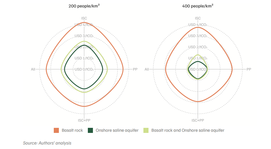
Figure ES1 presents the results of the 24 scenario analyses. The cost of building a CO₂ pipeline network is lowest when only onshore saline aquifers are used and highest when only basalt storage is used. This is because saline aquifers are geographically widespread, while basalt formations are concentrated mainly in Maharashtra and Madhya Pradesh, with some presence in adjoining states. We found that the cost of transport was USD 0.70–2.16 per tonne of CO₂ transported for the saline aquifers–only scenarios and USD 2.89–4.19 per tonne of CO₂ transported for the basalt-only scenarios, depending on the sources included.
When both basalt and saline aquifers were included, transport costs fell within the range of USD 0.87–2.51 per tonne of CO₂. This figure is slightly higher than the saline aquifers–only scenario because, in some cases, the model selected higher-capacity sinks when basalt and saline aquifers are both co-located, leading to fewer pipelines and longer injection durations. Transport costs varied depending on the overall volume of CO₂ transported. Therefore, the scenarios including power plants yielded lower costs than industry-only scenarios. Similarly, the scenarios with a population density of 400 people/km² yielded lower costs than those with 200 people/km² because the sinks are larger, have higher capacity, and are more contiguous, allowing for higher injection volumes. Overall, basalt-only scenarios result in higher transport costs than the saline aquifers–only scenarios. However, post-injection costs are significantly lower in basalt-only sinks (due to the formation of mineral carbonates, which can help eliminate leakage risks), which may offset the higher transportation costs.
Figure ES1. Cost of CO₂ transport is lowest in the case of saline aquifers
The methodology used in this analysis has the following limitations.
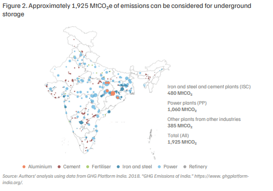
In 2018, India’s annual total emissions were approximately 3 GtCO₂ (gigatonnes of CO₂), of which around 73 per cent (2.1 Gt) were emitted by power plants and the industrial sector (including utility electricity generation, industries, captive power plants, and industrial process and product use emissions) (GHG Platform India 2018). Significant mitigation efforts will be required to limit the global temperature increase to 1.5°C and to meet India’s net-zero target by 2070. While India continues to promote renewable and alternative energy use to meet the growing energy demand in power systems and industries, legacy capacity in industries and the power sector that rely on fossil fuels cannot be easily abandoned before the end of their lifespans. As a result, fossil fuels will need to remain an integral part of India’s energy economy for several decades before the transition to green energy is complete.
To achieve net-zero by 2070, carbon capture and storage (CCS) will be indispensable. It is estimated that CCS can reduce economic losses by 23 per cent between 2030 and 2050 and by 32 per cent between 2050 and 2100 by reducing the pace of deployment of expensive low-carbon technologies and preventing the abandonment of operating assets (Chaturvedi and Malyan 2022). Additionally, the rate of increase in average power generation costs is lower in energy system modelling scenarios with CCS than in other energy modelling scenarios because CCS does not require changes to legacy fossil fuel–based capacity (Chaturvedi and Malyan 2022). To meet the 1.5°C temperature increase cap, India may have to inject 5.3–10 GtCO₂ by 2050 (Chaturvedi and Malyan 2022; Gambhir et al. 2021; Garg et al. 2017; Vishal et al. 2021). In addition to energy efficiency, renewable power, and alternative fuels, CCS could help mitigate up to 57 per cent of emissions from hard-to-abate sectors, such as steel, cement, and aluminium, because it is a significantly lower-cost alternative to carbon capture and utilisation (Elango et al. 2023; Nitturu et al. 2023).
India has a large storage potential of 317 GtCO₂, of which 144 Gt are in saline formations, 170 Gt in basalt, and the remaining in oil and gas and coal fields (Bakshi et al. 2023). CO₂ storage in basalt formations is unique because the injected CO₂ reacts with the basalt to form solid mineral carbonates over time, thereby eliminating the risk of long-term leakage. Since these geological formations can be far from major CO₂-emitting sources, a CO₂ transport network is needed. There are three major ways of transporting CO₂: by trucks, trains, or pipelines. The choice of transport mode depends on the distance, the quantity of CO₂ to be transported, the duration and frequency of transport, and whether the start and end points are stationary or mobile. Since our focus is on the long-term transport of large quantities of CO₂ from stationary sources to stationary CO₂ sinks, pipelines are the most economical choice in our analysis (Lu et al. 2020).
Studies on the design of an optimised CO₂ pipeline network typically recommend the hub-and-spoke model, a logistics strategy in which centralised collection at a specific place, or ‘hub’, serves as a focal point for redistribution to different locations, or ‘spokes’. This model helps manage and optimise network flow efficiently. However, there are two challenges with the hub-and-spoke model in the Indian context. First, Indian industrial and power generation facilities are distributed across the country, unlike in smaller countries, where they are concentrated in certain industrial clusters. This makes identification of hubs to support an industrial cluster difficult and possibly unnecessary. Second, in the context of optimising pipeline networks using a hub-and-spoke model, right-of-way (RoW) issues are not considered. RoW refers to the legal permission to lay and operate a pipeline through third-party-owned land. RoW can pose significant challenges, including land acquisition, compensation disputes, regulatory compliance and interference with existing infrastructure.
Pipeline construction projects in India are often significantly delayed because of RoW-related issues (Business Standard 2024; Department of Economic Affairs 2020; GlobalData 2024; Tewari 2024). Obtaining the necessary permissions to lay pipelines through forest areas, land demarcated for defence, coastal regulation zones, and government-owned lands is a complex and time-consuming process that often takes a year or more. There have been several instances in which pipeline construction had to stop due to RoW issues, sometimes delaying the project by many years, resulting in increased project costs and lost revenues (Economic Times 2020). To address such issues, in this study, we suggest an alternative conceptual approach in which we consider laying trunk CO₂ pipelines parallel to existing natural gas (NG) pipelines with RoW. Logically, this should reduce the time required to lay new pipelines and, hence, the overall cost of such projects. However, RoW will be necessary for spur pipelines that connect the source to the trunk line and the trunk line to the sink. This paper focuses on national-level network optimisation and estimates the costs and infrastructure required to transport CO₂ for CCS in India, using the RoW of an existing natural gas pipeline network to build new trunk CO₂ pipelines.
We suggest an approach of laying CO₂ pipelines along existing natural gas pipelines to limit land acquisition challenges and delays.
Globally, a few tools have been developed to optimise CO₂ capture, transport, and storage infrastructure. One paper reviewed all studies on CCS source–sink matching models conducted over the past 10 years and identified 16 model types based on 6 attributes: mitigation targets, carbon sources, carbon sinks (sequestration), transport networks, utilisation, and integration (synergy) (Zhang et al. 2022). However, no such study has focused specifically on India.
Garg et al. (2017) modelled CCS pipeline infrastructure with a focus on India. Such CCS mapping and network optimisation efforts clustered major CO₂ sources and sinks that are in proximity to one another. The most extensive source–sink mapping in India considered cluster sizes in the order of a few hundred kilometres (Garg et al. 2017). Garg et al. (2017) assumes that the straight-line transport of CO₂ within a cluster may be challenging due to barriers in obtaining the RoW for the entire network. The results of that study indicates that India has the potential to reduce approximately 780 MtCO₂ (million tonnes of CO₂) annually at a cost of less than USD 60 per tonne of CO₂ for 30 years by implementing CCS.
Another study focused on linear programming-based source–sink mapping in eastern India to reduce CO₂ emissions from thermal power plants (Jain et al. 2013). The authors conducted a spatial analysis of the proposed pipeline route along a railway network, which may not be particularly useful for creating a pipeline network for CCS. In addition to RoW-related issues, given alignment with railway lines, vibrations from moving trains may risk the safety of the system (Jain et al. 2013).
One source–sink matching model, when applied to large, concentrated CO₂ sources located within 20 km of geological storage, accounted for only 3 per cent of India’s emissions (Beck et al. 2013). Other studies have provided rough estimates of the cost of a CCS supply chain, but do not focus much on network optimisation (Sharma and Yuan 2021).
In this study, we optimised the CO₂ transport network for CCS in India, considering the RoW of the existing NG pipeline network to estimate CO₂ sequestration potential and cost. We considered all major point sources of emissions, including 486 plants from the top two industrial sectors (iron and steel, and cement) and 214 power plants. In the long run, we expect only the steel, cement and power sectors to use CCS, as other sectors can transition to green alternatives. However, there may still be a need to store CO₂ from other sectors, such as aluminium, fertiliser, and refineries, during the transition phase. Adding the other industrial sectors increased the number of source facilities in this study to 765. We also considered the possibility of using onshore saline aquifers, basalt formations, or both, as sinks. We did not evaluate oil and gas and coal fields because their total storage potential is low. Overall, we aimed to understand the various possible configurations of pipeline networks, depending on the emission sources and sinks chosen and the resulting transport costs.
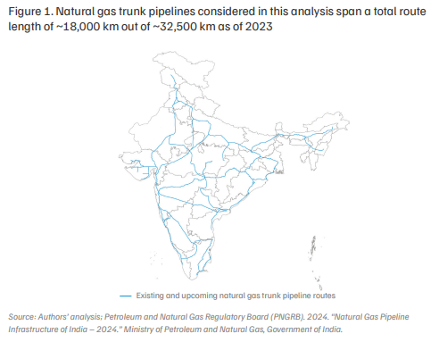
To evaluate the proposed CO₂ transport pipeline network, we leveraged the RoW for the existing and under-construction NG pipeline network. The analysis excludes crude oil (~11,000 km), petroleum products, and liquified petroleum gas (LPG) pipelines (~23,000 km) (PPAC 2024). The optimal solutions for a CO₂ transport pipeline network may be shorter in length and thus cost less to build if crude oil, petroleum product, and LPG pipelines were included in the analysis. However, due to a lack of geographic information system (GIS) data and limited computing power, we included only the RoW of approximately 18,000 km of the NG network’s trunk pipelines, as shown in Figure 1. The 18,000 km network length indicates the route length (the RoW along the trunk pipelines), and not the length of the pipelines (which total to ~32,500 km, because, in many routes, there are multiple NG pipelines that run in parallel, such as the Hazira–Vijaipur–Jagdishpur pipeline section, where three pipes are laid in parallel).
We designed an optimised pipeline network for transporting CO₂ from 765 power and industrial plants to potential onshore underground storage sites.
We refer to all new CO₂ pipelines laid down using the RoW for the existing NG pipeline network as trunk pipelines (to mean the same as associated routes). We also analysed how much of the new CO₂ spur pipelines overlap with existing NG spur pipelines Spur pipelines carry CO₂ from the source to the trunk pipelines and from the trunk pipelines to the sinks.
Our model used the following four-step process to build the CO₂ pipeline network.
i. Find the shortest/cheapest path between each source–sink pair
First, we mapped the existing, under-construction, and approved NG pipeline routes on GIS software using data provided by Genesis Ray (2022). Before using this as an input in our model, the spur pipeline routes of the existing NG pipeline network were removed to reduce complexity and runtime. The resultant network (or graph data structure) consisted of linear splines with a total route length of approximately 18,000 km. To find the shortest possible path between each source and sink, we first defined a weighted graph data structure consisting of vertices and edges. The vertices were defined such that the route between any two adjacent vertices is a linear edge of length less than or equal to 100 km.
The values or weights of the edges were defined as follows: If two vertices are directly connected by an NG pipeline route, the weight of that edge is simply taken as the length of that route. Otherwise, the weight of the edge is equal to the Euclidean distance multiplied by the RoW factor. The RoW factor was introduced to discourage the model from building pipelines when an existing NG RoW is nearby. This factor needs to be large enough to maximise the selection of the existing RoW routes.
The existing NG trunk pipeline routes are not necessarily connected to the existing sources and future sinks. Therefore, the graph trunk pipeline routes were extended to include the sources and sinks, with new edges. The weights assigned to these new edges were also defined as the product of the Euclidean distance and the RoW factor, since they will all become new spur pipelines. As sinks are regions and not points, the distance from a vertex to a sink was defined as the shortest distance between the vertex and the sink boundary.
The weighted graph was used as the input for the Floyd–Warshall algorithm to compute the shortest distances (based on edge weights) between each source and sink. The Floyd–Warshall algorithm is one of the most efficient algorithms for finding the shortest paths between points in a weighted graph and is used to solve network and connectivity problems in which all the nodes in a network are connected. The algorithm output is a table that comprises the weighted lengths of the shortest paths between each source–sink pair.
ii. Optimally allocate the CO₂ flow rate
In this step, we used a linear programming-based model to connect each source to a sink (based on the shortest paths identified in Step 1, such that the average cost of CO₂ transport across the entire network was minimised). The model used the following inputs:
• A matrix containing the shortest/cheapest distances from each source to each sink for all source–sink combinations
• Yearly emissions from each source
• Storage potential of each sink
• Duration for which we need to optimise, i.e. the number of years over which CO₂ will be injected in the sink
Additional decision variables were included in the model to represent the CO₂ flow rate from each source to each sink. The model allocates a positive value to only one of the variables for each source– sink combination when an optimal solution was found, indicating that only one of the many possible connections was made between a source and a sink. An objective function subject to constraints allocated CO₂ from each source to a given sink based on the minimised cost of transport cost, as shown here:
Objective function
The objective was to minimise the total transport cost. Ideally, the pipelines would be represented as a number of discrete standard pipeline sizes. However, this type of representation would require a large number of continuous and binary variables and constraints in a mixed-integer linear programming formulation, significantly increasing the computational resources required. Instead, our function represented the pipelines as a single linear function (passing through the origin) of cost and pipeline capacity (flow rate) for a given length, ensuring that the cost estimate yielded by the model is realistic (Middleton et al. 2020). The cost of each pipeline was directly proportional to the product of flow rate and pipeline length. Thus, our objective function minimised the sum of the products of the flow rate and the weighted length for each source–sink connection, as described in Step 1. Mathematically, the objective function can be represented as:
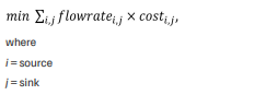
Note that although we used a simplified pipeline cost function for optimisation, the actual pipeline cost function (without simplification) was used to calculate the final costs, as described in Step 4.
Constraints
• The CO₂ flowing out of a source should be equal to its emissions
• The total CO₂ flowing into a sink in a decided time period should be less than the capacity of that sink
![]()
where
life = assumed lifespan of the pipeline (25 years)
The output of this linear programming model provided an allocation of the CO₂ flow rate, which minimised the total cost of the pipeline network using the simplified cost function with a zero y-intercept. The output obtained in this step established an independent connection from each source to the chosen trunk pipeline and further to the sink through that trunk pipeline. To leverage economies of scale and reduce costs, it was practical to aggregate the flows going through overlapping or similar routes of spur pipelines. Hence, the solution obtained in this step was suboptimal.
iii. Minimise the spur pipeline route length
To address suboptimality and consolidate multiple spur pipelines into a single pipeline, we further reduced the total length of the spur pipelines using Kruskal’s algorithm, which is highly efficient when the number of splines is minimal/sparse (GeeksforGeeks 2023). In this step, we combined multiple spur pipelines in the same vicinity and connecting to the same trunk pipeline into a single spur pipeline. Therefore, the output was a reduced length of spur pipelines in the overall network.
iv. Identify the overlap of CO₂ spur pipelines with existing NG spur pipelines
Step 1 excluded the existing NG spur pipeline routes to keep the computation process manageable. However, the RoW of the existing NG spur pipelines would reduce the land access burden for the CO₂ 2. Average cost break-up provided by a large gas pipeline operator in India. spur pipelines, similar to trunk pipelines. Therefore, in this step, the new CO₂ spur pipelines were overlaid on the existing NG spur pipelines to identify overlaps. For those spur pipelines that overlap, we assumed zero RoW cost. The pipeline network obtained at this stage is the final network, for which the total cost was again calculated using the actual cost vs. flow rate function based on the FECM/NETL CO₂ Transport Cost Model developed by the National Energy Technology Laboratory (Morgan et al. 2023) instead of the simplified function used in Step 2. Since material costs are only one component of the total costs, total costs were assumed to be a product of the material costs based on the assumptions mentioned in Section 3.1. For the trunk pipelines, we assumed zero RoW costs.
The actual cost of the final pipeline network may not be the absolute minimum possible given the simplifications assumed, but it is a good enough approximation to guide the future efforts of all relevant stakeholders and policymakers.
This section outlines the key assumptions made to estimate the pipeline cost curve for CO₂ transport.
• Inlet pressure: 2,200 psig (Morgan et al. 2023)
• Outlet pressure: 1,200 psig (Morgan et al. 2023)
• Temperature: 32°C (slightly above the critical temperature of CO₂) (Witkowski et al. 2014)
• Pipeline length between pumps: 150 km
• Capacity factor: 85 per cent (Morgan et al. 2023)
• Material: API 5L X70 steel (Witkowski et al. 2014)
This configuration ensured that CO₂ remained in a supercritical state, which is essential for efficient transport as it behaves as a compressible fluid. We used the FECM/NETL CO₂ Transport Cost Model to estimate the minimum pipeline diameter and corresponding thickness required for different flow rates (Morgan et al. 2023).
The material cost of the pipeline was calculated using prevailing steel prices in India, assuming a 50 per cent volume discount (Trident Steel & Engg. Co. 2024). We divided the total pipeline cost into four major components: material (40 per cent), laying (30 per cent), RoW (15 per cent), and miscellaneous (15 per cent).2 We estimated the total pipeline-laying costs using the material cost estimate and scaled them up based on the percentage of material costs in the total costs.
To estimate the amount of CO₂ to be transported in the pipeline system, we assumed that 75 per cent of the total power plant emissions and 50 per cent of all industrial emissions can be captured and stored underground permanently. In the case of coal thermal power plants, there are a few alternatives for mitigating emissions, and the bulk of the emissions must be mitigated either through carbon capture and utilisation or underground storage. In contrast, industrial sectors have multiple issues, such as energy efficiency, renewable power, and alternative-fuel mitigation options, before the residual emissions can be addressed. Hence, for industrial sectors, we assumed that only 50 per cent of the CO₂ can be captured for storage.
We assumed that 75% of power plant emissions and 50% of industrial emissions can be captured and stored underground permanently.
We considered multiple scenarios to help relevant stakeholders make informed decisions regarding goals, planning, and research. Each scenario includes three variables: the sources (industries and power sector) considered, the type of sinks considered, and the constraint parameters that limit the feasible storage potential.
Industries considered
We considered plants from the following industries as sources:
• Aluminium
• Cement
• Fertiliser
• Iron and steel
• Power
• Refineries
Furthermore, industries were grouped based on their ability to reduce emissions using methods other than CCS and on the remaining life of existing plants. The following three source groupings were considered:
• Power plants (PP)
• Iron and steel and cement plants (ISC)
• All plants from all industries (All)
Power plants were considered separately because many may be shut down over time as the overall power system moves towards renewable energy sources. In such a scenario, dedicated trunk pipelines to potentially end-of-life power plants may not make sense. However, at this time, there is no clarity on how power plants will transition in the future; hence, we assumed the continuation of operations for the existing power plants. Iron and steel and cement plants were also considered separately because a significant portion of their process emissions cannot be reduced through other interventions, and legacy plants have significant residual life remaining. Thus, there are four possible choices when considering the sources:
• Power plants (PP)
• Iron and steel and cement plants (ISC)
• Power and ISC plants (ISC + PP)
• All plants (All)
Figure 2 presents the total emissions and geographical locations of all source categories considered in this analysis.
Type of sinks considered
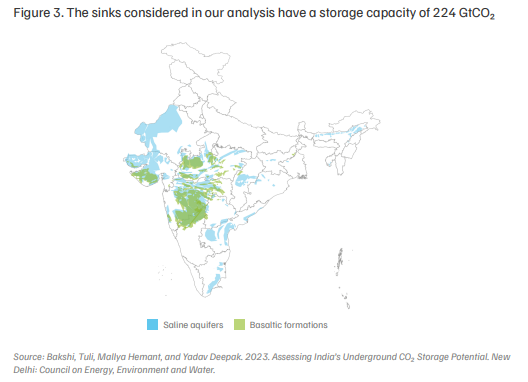
We only considered onshore sinks in our analysis. Since onshore basalt and saline aquifers constitute approximately 99 per cent of India’s onshore storage capacity, only these two types of sinks were considered.
There are three possible choices in terms of sinks:
• Basalt only (170 Gt)
• Saline aquifers only (54 Gt)
• Basalt and saline aquifers (224 Gt)
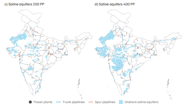
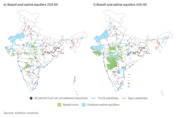
Figure 3 presents the spatial distribution of these sinks (Bakshi et al. 2023).
Constraint parameters
Various above-ground challenges considerably influence the realisable underground storage potential. Population density is one such factor. The realisable storage potential increases when we allow more densely populated areas to be used as storage sites. According to a previous study by CEEW, there are two inflexion points on the curve of storage potential vs population density at 200 and 400 people/km2, where the area available and storage potential change substantially (Bakshi et al. 2023). Thus, for each of the three choices of sinks mentioned above, the storage potential at both population density levels was evaluated. Population density is a good indicator of local resistance and other above-ground challenges.
Population density is also a significant factor in the safe design and construction of pipelines. The ASME B31.8 Code for Pressure Piping (2003) is a commonly used standard for design, construction and maintenance requirements. The code defines ‘Location Class’ based on the number of buildings intended for human occupancy along any 1-mile section of a pipeline. Location Class 1 applies to a section that has 10 or fewer buildings and reflects areas, such as “wasteland, deserts, mountains, grazing land, farmland, and sparsely populated areas”. Location Class 2 applies to a section that has more than 10 but fewer than 46 buildings and reflects “fringe areas around cities and towns, industrial areas, etc.” Location Class 3 applies to a section that has 46 or more buildings and reflects areas, such as “suburban housing developments, shopping centres, residential areas, industrial areas, and other populated areas”. Location Class 4 includes “areas where multistorey buildings are prevalent, where traffic is heavy or dense, and where there may be numerous other utilities underground”.
The allowable pressure decreases with increasing location class; alternatively, pipe thickness must be increased for the same pressure with increasing location class. In the context of our analysis, storage sites may be possible only in Location Classes 1 and 2, which have a population density of approximately less than 200 people per km2 and Location Classes 2 and 3, which have a population density of approximately less than 400 people per km2 . In some instances, the pipeline network may pass through Location Class 4.
Considering all the possible combinations of these sources, sinks, and population density levels, 24 combinations can be created. We did not include location classes because of a lack of granular data at the sectional level of pipelines.
We ran 24 scenarios to evaluate the CO₂ pipeline network and determine the associated costs. Table 1 presents details on the lengths of pipeline routes to be built either on existing RoW or new RoW. The pipeline lengths are longer because some sections have multiple pipes.
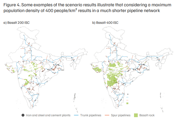
Saline aquifers are a sink resource found across the country; hence, the pipeline network with the saline aquifers–only scenario yielded the smallest network size for all source combinations except for ISC, where the network size in the basalt and saline aquifers scenario was marginally smaller. Correspondingly, we found that the cost per tonne of CO₂ transported was lowest in the saline aquifers–only scenario and fell within the range of USD 0.70–2.16 per tonne of CO₂ transported, depending on the sources included in the scenarios.
Basalt resources are largely limited to Maharashtra and Madhya Pradesh, with some resources in the adjoining states. Therefore, the CO₂ pipeline network obtained in the basalt-only scenario was much larger than in the saline aquifers–only scenario. Hence, the cost of transport was the highest in the basalt-only scenario and fell within the range of USD 2.89–4.19 per tonne of CO₂ transported, depending on the sources included in the scenarios.
When basalt and saline aquifers were considered, the pipeline lengths were marginally higher than in the saline aquifers–only scenario. The reason is that, sometimes, the model selected higher-capacity sinks to reduce pipeline length when basalt and saline aquifers were co-located, rather than the same sinks used in the saline aquifers–only scenario. The cost of transport in the basalt and saline aquifers scenario fell within the range of USD 0.87–2.51 per tonne of CO₂ transported, depending on the sources included. Table 1 summarises all cases, while Figure 4 presents a few selected cases.
The cost of transport was generally the lowest when all the emission sources were included in the analysis. Power plants have a significant influence on transport costs; in general, the cost in the power plants scenario was among the lowest across all sink types. Finally, the scenarios with sinks at 400 people/km² yielded lower costs than those with 200 people/km2 scenarios because the sinks are larger and have higher capacity in the former case. All cost calculations utilised the actual pipeline length and not route lengths. Route lengths are relevant for RoW cost calculations, while pipeline lengths are relevant for material costs.
The cost of transporting CO₂ to both basalt and saline aquifers was USD 0.87–2.51 per tonne of CO₂, depending on the sources included.
| S. no. | Emission source | Total emissions (Mtpa) | Sink | Population filter (people/ km²) | Spur routes length (km) with RoW | Spur routes length (km) without RoW | Trunk route total length (km) | Total pipeline length (km) | Spur material annualised CAPEX (million USD) | Trunk material annualised CAPEX (million USD) | Total annual cost (million USD) | USD/ tonne CO2 |
|---|---|---|---|---|---|---|---|---|---|---|---|---|
| 1 | ISC | 239.6 | Basalt | 200 | 803 | 7,877 | 10,105 | 18,785 | 78 | 232 | 1,004 | 4.19 |
| 2 | ISC | 239.6 | Saline aquifers | 200 | 2,364 | 6,319 | 5,892 | 14,575 | 53 | 105 | 519 | 2.16 |
| 3 | ISC | 239.6 | Basalt and saline aquifers | 200 | 2,453 | 7,620 | 7,217 | 17,290 | 69 | 113 | 601 | 2.51 |
| 4 | ISC | 239.6 | Basalt | 400 | 2,036 | 6,203 | 9,295 | 17,534 | 61 | 220 | 900 | 3.76 |
| 5 | ISC | 239.6 | Saline aquifers | 400 | 1,799 | 4,757 | 3,950 | 10,506 | 35 | 13 | 167 | 0.70 |
| 6 | ISC | 239.6 | Basalt and saline aquifers | 400 | 2,249 | 4,676 | 3,521 | 10,446 | 42 | 51 | 311 | 1.30 |
| 7 | PP | 795.8 | Basalt | 200 | 1,850 | 5,194 | 12,043 | 19,087 | 174 | 694 | 2,779 | 3.49 |
| 8 | PP | 795.8 | Saline aquifers | 200 | 2,263 | 4,615 | 8,654 | 15,532 | 110 | 297 | 1,319 | 1.66 |
| 9 | PP | 795.8 | Basalt and saline aquifers | 200 | 2,200 | 5,608 | 11,152 | 18,960 | 156 | 353 | 1,659 | 2.09 |
| 10 | PP | 795.8 | Basalt | 400 | 2,002 | 4,464 | 10,674 | 17,140 | 142 | 625 | 2,448 | 3.08 |
| 11 | PP | 795.8 | Saline aquifers | 400 | 1,877 | 3,687 | 4,209 | 9,773 | 74 | 130 | 673 | 0.85 |
| 12 | PP | 795.8 | Basalt and saline aquifers | 400 | 2,054 | 3,992 | 4,329 | 10,375 | 79 | 130 | 690 | 0.87 |
| 13 | ISC + PP | 1035.4 | Basalt | 200 | 3,371 | 10,555 | 12,790 | 26,716 | 252 | 817 | 3,444 | 3.33 |
| 14 | ISC + PP | 1035.4 | Saline aquifers | 200 | 3,256 | 10,355 | 10,025 | 23,636 | 194 | 361 | 1,821 | 1.76 |
| 15 | ISC + PP | 1035.4 | Basalt and saline aquifers | 200 | 3,412 | 10,660 | 11,477 | 25,549 | 230 | 427 | 2,157 | 2.08 |
| 16 | ISC + PP | 1035.4 | Basalt | 400 | 3,432 | 9,205 | 11,457 | 24,094 | 210 | 725 | 3,004 | 2.90 |
| 17 | ISC + PP | 1035.4 | Saline aquifers | 400 | 2,846 | 7,434 | 5,397 | 15,677 | 116 | 153 | 894 | 0.86 |
| 18 | ISC + PP | 1035.4 | Basalt and saline aquifers | 400 | 3,118 | 7,646 | 5,116 | 15,880 | 124 | 158 | 941 | 0.91 |
| 19 | All | 1126.5 | Basalt | 200 | 3,748 | 10,996 | 16,627 | 31,371 | 280 | 910 | 3,832 | 3.40 |
| 20 | All | 1126.5 | Saline aquifers | 200 | 3,904 | 10,315 | 10,418 | 24,637 | 208 | 396 | 1,982 | 1.76 |
| 21 | All | 1126.5 | Basalt and saline aquifers | 200 | 3,690 | 10,801 | 12,157 | 26,648 | 246 | 464 | 2,327 | 2.07 |
| 22 | All | 1126.5 | Basalt | 400 | 3,893 | 9,143 | 11,880 | 24,916 | 224 | 790 | 3,257 | 2.89 |
| 23 | All | 1126.5 | Saline aquifers | 400 | 3,301 | 7,510 | 5,979 | 16,790 | 118 | 170 | 954 | 0.85 |
| 24 | All | 1126.5 | Basalt and saline aquifers | 400 | 3,487 | 7,605 | 5,548 | 16,640 | 133 | 179 | 1,038 | 0.92 |
• Availability of RoW: We assumed that the existing pipeline network has sufficient space to lay a parallel CO₂ pipeline across the entire network. However, this may not hold in practice, and several sections may require additional RoW. Expanding the existing RoW may be easier than acquiring land for a new RoW. Nonetheless, our analysis indicated a shorter pipeline length and lower cost than is likely in the real world.
• Exclusion of crude oil and petroleum product pipelines: This analysis only relied on the RoW of NG pipelines. Adding crude oil and petroleum product pipelines would increase the total length of existing RoW, thereby reducing the network length for new CO₂ pipelines. Accordingly, the overall pipeline length was overestimated in our analysis.
• Euclidean distance of spur pipelines: We used the actual network pathways of existing NG pipelines. However, spur pipelines were estimated using straight-line Euclidean distance, which does not reflect real-world conditions. Hence, the spur pipeline lengths were underestimated in our analysis.
• Cost breakdown for the pipeline network: We relied on a rough breakdown of cost components (materials, laying, RoW, and miscellaneous). In practice, this breakdown will vary across different pipeline sections. We assumed that, on average, the costs would hold at the national level. However, we could not determine uncertainty due to the lack of granular, section-level data.
• Storage capacity of sinks: The CO₂ storage capacity of the sinks is an approximation, and there is inadequate detailed geological data to ascertain the exact storage potential. Hence, if there were a change in the storage capacity of the sinks, the pipeline network would also change; however, this uncertainty cannot be determined at this stage.
• Emissions trajectory: We used a static emissions profile for power plants and industrial facilities considered in this analysis. However, overall emissions are expected to grow over time. Depending on the change in location of emissions abatement (due to plant closures) or the emergence of new emission sources (due to new plant establishment or capacity expansion), the pipeline network would evolve over time. However, this aspect was not captured in our analysis.
In this study, we proposed a practical solution for transporting CO₂ in the Indian context and estimated the transport costs. In this section, we offer guidance for policymakers and relevant stakeholders. The results are not intended to be implemented as they are, since there are practical constraints and considerations that only the implementing entities can incorporate. Our recommendations are intended to enable the development of a CO₂ pipeline network in the country and are presented as follows.
• Develop a national CCS policy: A crucial first step in developing a CCS ecosystem is identifying the ministry that will own the mandate. Subsequently, a national policy needs to be developed to encourage the development of a CCS ecosystem to capture, transport, and permanently store CO₂, with underground storage as one option. It is also important to establish a regulatory authority to monitor infrastructure development and pricing rules for underground storage, and to safeguard public interests.
• Determine how much of the existing RoW can be utilised: In this study, we assumed that all existing RoW would have sufficient space to accommodate new CO₂pipelines, which may not be the case in practice. A separate study is needed to determine which sections of the existing RoW for NG, crude oil, and petroleum product pipelines have sufficient space to deploy new CO₂pipelines. This should include the length of such sections and the pipeline capacity (diameter) that can be deployed.
• Amend the Petroleum and Minerals Pipelines (Acquisition of Right of User in Land) Act, 1962, to include CO₂: Currently, the Act only provides for the acquisition of land for transporting petroleum and minerals. Hence, it is not possible to use existing RoW or acquire new RoW to lay new CO₂pipelines. Additionally, modifying existing NG pipelines to carry CO₂ in the future is not possible. Therefore, the Act needs to be amended to allow the following: use of the RoW of existing petroleum and minerals pipelines for laying new CO₂pipelines; acquisition of new RoW for laying new CO₂pipelines; and provisions for converting RoW for petroleum or minerals to RoW for CO₂ in the future.
• Evaluate how much CO₂will need to be transported: The cost of transporting CO₂ depends on the capacity of the pipeline network to be developed, which depends on the amount of CO₂ to be transported. It is expected that India will continue to use fossil fuels despite the rapid growth in renewable energy sources, and national emissions will peak only in the mid2040s (Chaturvedi and Malyan 2022). We can also expect the addition of new plants based on fossil fuels over the next two decades to increase national emissions. Conversely, some plants will be shut down or transitioned to clean fuels, thus reducing national emissions. In this study, we assumed the source locations and their emissions to be static (i.e., they do not change over time), but further analysis is required to forecast changes in sources; this would make our results dynamic and more realistic. Hence, an evaluation is needed to estimate how much CO₂must be transported annually and permanently stored underground until India achieves net-zero.
• Identify high-source-density corridors for pipeline development: This study estimated the cost of CO₂ transport for an entire pipeline network. However, certain corridors have a high density of CO₂ source, resulting in substantially lower transport costs than our estimate – specifically, the corridor in eastern India, running through West Bengal, Odisha, and Jharkhand, and into Chhattisgarh. Similar corridors should be incrementally identified and prioritised in building the network.
CO₂ is captured at the source (such as a power plant or steel mill), compressed to a supercritical state above its critical temperature and pressure, and transported through dedicated pipelines to a storage site. In the supercritical state, CO₂ behaves as a compressible fluid, enabling efficient high-volume transport. The pipeline network consists of large-diameter trunk pipelines, carrying CO₂ from major source areas to major sink areas, and smaller-diameter spur pipelines, connecting individual sources or sinks to the trunk pipelines. Pumping stations are installed at regular intervals (typically every 150 km) to maintain pressure throughout the system.
Right-of-way (RoW) refers to the legal authorisation granted to a project to build and maintain infrastructure on a continuous strip of land. In India, obtaining RoW for a new pipeline requires land acquisition, compensation negotiations with landowners, and regulatory approvals across multiple jurisdictions, often delaying projects by several years. Obtaining permissions to lay pipelines through forest areas, defence lands, coastal regulation zones, and government-owned lands can each take a year or more. This study proposes using the existing RoW of NG pipelines to lay new CO₂ pipelines in parallel, which would significantly reduce these barriers.
This study estimates that the cost of transporting CO₂ through a pipeline network using the RoW of existing NG pipelines ranges from USD 0.70 to USD 4.19 per tonne of CO₂, depending on the emission sources included and the storage sites used. Saline aquifer-only scenarios are the least expensive (USD 0.70–2.16 per tonne), while basalt-only scenarios are the most expensive (USD 2.89–4.19 per tonne). These transport costs are relatively low compared with capture costs, which typically range from USD 30 to USD 100 per tonne, and represent a small fraction of the total CCS chain cost.
Several regulatory and policy actions are required. First, India currently lacks a national CCS policy, and identifying the ministry that will own the mandate is a crucial first step. Second, the Petroleum and Minerals Pipelines (Acquisition of Right of User in Land) Act, 1962, needs to be amended to allow CO₂ pipelines to use existing NG and petroleum pipeline RoWs, and to enable the acquisition of new RoW for CO₂ pipelines. Third, a regulatory authority needs to be established to oversee infrastructure development and safeguard public interests. Finally, an assessment of how much of the existing RoW across NG, crude oil, and petroleum product pipelines can accommodate new CO₂ pipelines is urgently required.
Carbon capture and storage (CCS) is a technology that captures CO₂ emissions from industrial facilities or power plants, compresses them into a supercritical state, and transports them through pipelines to underground geological formations for permanent storage. Suitable storage formations include saline aquifers, basalt formations, and depleted oil and gas fields. CCS is widely recognised as an essential tool for achieving net-zero emissions, particularly for sectors where alternative decarbonisation pathways are limited or prohibitively expensive.
India has committed to achieving net-zero emissions by 2070. However, the energy transition will take several decades, during which fossil fuel-based power plants and heavy industries will continue to emit CO₂. CCS is essential for addressing these residual emissions, particularly from hard-to-abate sectors such as iron and steel, cement, and aluminium, where process emissions cannot be fully eliminated through energy efficiency or renewable energy alone. CEEW modelling indicates that CCS could reduce India’s economic losses by 23 per cent between 2030 and 2050 and by 32 per cent between 2050 and 2100, and could mitigate nearly 60 per cent of emissions from these sectors.
CCS involves permanently storing captured CO₂ in deep geological formations underground, while carbon capture and utilisation (CCU) converts captured CO₂ into useful products such as fuels, chemicals, or construction materials. CCS is generally more cost-effective for large-scale emissions reduction, since underground storage is significantly cheaper than the processes required for utilisation. However, CCU can offer economic co-benefits through the sale of derived products. Both approaches are complementary, and India’s decarbonisation pathway may need to deploy both, with CCS handling the bulk of industrial and power sector emissions.
India has three main types of onshore geological formations suitable for CO₂ storage. Saline aquifers (144 GtCO₂ capacity) are geographically widespread and are the least expensive storage option due to their proximity to emission sources. Basalt formations (170 GtCO₂ capacity) are concentrated primarily in Maharashtra, Madhya Pradesh, and adjoining states. Oil and gas fields and coal formations have a comparatively limited storage potential. Together, India’s total onshore storage potential is estimated at approximately 317 GtCO₂, which far exceeds the country’s projected cumulative emissions over the coming decades.
Basalt formations have a unique geochemical property: when CO₂ is injected into basalt, it reacts with the rock to form solid mineral carbonates over time, a process known as mineral carbonation. This converts the gaseous CO₂ into a stable solid form, virtually eliminating the risk of long-term leakage. Although transport costs to basalt formations are higher due to their geographic concentration, the significantly lower post-injection monitoring and leakage-risk costs may make basalt storage more economical over the full project lifecycle.
Hard-to-abate sectors are industries in which decarbonisation is technically difficult or prohibitively expensive using current technologies. These include iron and steel, cement, aluminium, and chemicals. A large share of their emissions arises from chemical processes rather than from energy use alone, meaning that switching to renewable energy does not eliminate these process emissions. CCS is currently one of the few viable options for addressing process emissions at scale. India’s iron and steel and cement plants alone account for approximately 480 million tonnes of CO₂ per annum that could potentially be captured and stored underground.
How Secure is India’s Energy Future?
Unlocking the Potential for a Gas-Based Economy in India
Advancing India’s Green Steel Transition
Bharat Cleantech Manufacturing Platform: Green Hydrogen Indigenisation Pathways
How Will India’s Vehicle Ownership Grow?