Council on Energy, Environment and Water Integrated | International | Independent
Suggested Citation: Jalan, Ishita and Hem H. Dholakia. 2019. What is Polluting Delhi’s Air? Understanding Uncertainties in Emissions Inventory. New Delhi: Council on Energy, Environment and Water.
Fixing Delhi's air quality requires a deep understanding of the sources that contribute to air pollution. Despite multiple source apportionment studies specific to Delhi NCR, policymakers can’t design an effective action plan due to varying estimates. This study brings clarity on the existent discrepancies and attempts to understand the gaps and opportunities to develop emissions inventory for source apportionment studies.
Our study focuses on five emission inventory studies (CPCB 2010; IIT Kanpur 2015; TERI 2018; SAFAR 2018; Guttikunda 2018) on Delhi NCR. It draws comparisons between emissions inventories for ten sources of air pollution for PM10 and PM2.5.
Sector-wise contribution to PM2.5 (%)
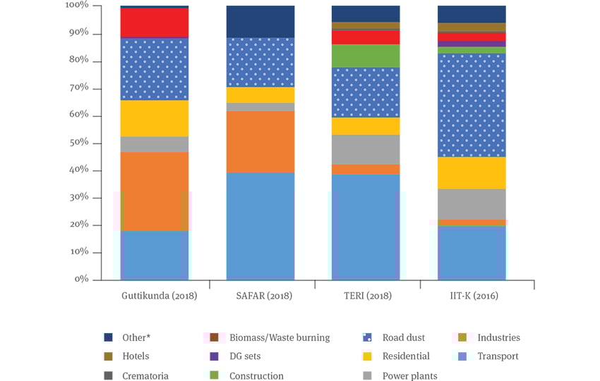
Source: CEEW analysis, 2019
Sector-wise contribution to PM10 (%)
Source: CEEW analysis, 2019
Why Do Emissions Inventories Currently Vary?
In India, every year, air pollution causes 1.24 million deaths. In Indian cities, most of the year, the average concentration of particulate matter (PM) exceeds Central Pollution Control Board (CPCB) standards. Making decisions on mitigation and control requires an understanding of air pollution sources. Source apportionment estimates the contribution of each source.
The process uses two methodologies - top-down and bottom-up. The two methodologies complement each other in cross-checking and validating the source apportionment analysis; therefore, it is advised to use both for a region. Delhi is popular in the narrative of air pollution, and it has been covered extensively by source apportionment studies (CPCB 2010; IIT Kanpur 2016; TERI 2018; SAFAR 2018; Guttikunda 2018).
These studies have played an instrumental role in describing the variety of sources that contribute to air pollution in Delhi and the National Capital Region (NCR), but their estimates differ significantly. Given that source apportionment information guides pollution mitigation policy and actions, differences can make the determination of exact sources uncertain and air quality improvement measures ineffective.
By comparing the existing emissions inventories for Delhi or NCR, this study aims to explain the differences in these estimates. To detail these differences, we focus on PM10 and PM2.5 in transport, industries, power plants, road dust, and construction - the five major contributing sectors. An emissions inventory uses the bottom-up method and forms the basis for a source apportionment study. A dispersion model is used to calculate the distribution of pollution using the emissions inventory and meteorological data as input parameters.
The biggest contributor of PM2.5 is the transport sector; its contribution ranges from 17.9 per cent to 39.2 per cent. Road dust is the second largest source of PM2.5; it contributes between 18.1 per cent and 37.8 per cent. It also contributes 35.6 per cent to 65.9 per cent of PM10 as the largest source. Similar trends exist for other sectors. The differences are due to each study’s domain area; year; sampling season chosen; and methodologies of sampling, estimation, and emissions factors. These factors explain the discrepancies only partially, however; emissions inventories are different for other, unexplained reasons.
To improve the understanding of air pollution and formulation of policy, several changes are necessary. Information on sampling frame and sample details needs to be transparent. Uncertainty should be quantified to explain the spread of observations for a sector. Multipleyear inventories would capture the dynamic nature of air pollution and enable accurate, realtime information. Common regulatory guidelines would help in building robust inventories. Source apportionment based on emissions inventories and dispersion modelling should be reconciled with receptor modelling to enable convergence between the modelling and measurement approaches.
Worldwide, 9 out of 10 people breathe polluted air 1 Air pollution poses one of the biggest risks to human health. About 29 per cent of deaths and disease due to lung cancer; 43 per cent from chronic obstructive pulmonary disease; and 25 per cent of deaths due to heart disease and stroke2 are attributable to ambient air pollution. The Global Burden of Disease 2017 reported 1.24 million deaths can be linked to air pollution (Madhipatla et al., 2018).
Pollution is one of the largest causes of morbidity and mortality; it also puts a great burden on the Indian economy, causing losses of approximately $56 billion in 2013 alone (World Bank, 2016). Air quality management measures, short- and long-term, require an understanding of pollution sources and of the temporal and spatial distribution of pollutants. Several studies have compiled emissions inventories for India and other Asian countries. Delhi, among the most polluted cities worldwide, and often discussed in the popular narrative, is one of the most studied regions in India in the context of air pollution. This study compares inventories developed for Delhi and its surrounding regions.
An emissions inventory of a given study region is a stock of all its pollution-emitting sources, such as vehicles, industries, power plants, road dust, construction dust, residential, diesel generator (DG) sets, biomass/waste burning, crematoria, and hotels. Developing an emissions inventory is a step in the bottom-up approach of apportioning sources. Apart from direct emissions estimates, emissions in these sectors are calculated by multiplying energy consumption with the emissions factor to derive the pollution per unit energy consumed. This information is an input to the dispersion model, which converts pollution estimates (mass/year) to ambient concentration (mass/volume). Ambient concentration is directly comparable to source apportionment estimated using receptor modelling.
Several emissions inventories have been developed for Delhi or larger areas that include the NCR.4 These inventories contribute to source apportionment studies. Often, this drive pollution control decision making in the region by statutory agencies such as the Environment Pollution Prevention and Control Authority (EPCA), Central Pollution Control Board (CPCB), and other State Pollution Control Boards (SPCB).
Few studies compare emissions inventories across anthropogenic and combustionrelated emissions of air pollutants or analyse uncertainties in inventory measurement (input parameters). Therefore, the extent of uncertainty in source apportionment (output parameter) is unclear. In this note, we compare the emissions inventories for Delhi and the NCR.

This work relies on existing emissions inventories that provide estimates for Delhi or the NCR. The NCR encompasses the entire national Capital Territory (NCT) of Delhi (1,483 square kilometres (sq km) and a few districts of Haryana (thirteen), Uttar Pradesh (eight), and Rajasthan (two) (totalling 53,600 sq km).
The 13 districts of Haryana are Faridabad, Gurugram, Mewat, Rohtak, Sonepat, Rewari, Jhajjhar, Panipat, Palwal, Bhiwani (including Charkhi Dadri), Mahendragarh, Jind, and Karnal. The eight districts of Uttar Pradesh are Meerut, Ghaziabad, Gautam Budh Nagar, Bulandshahar, Baghpat, Hapur, Shamli, and Muzaffarnagar. The two districts of Rajasthan are Alwar and Bharatpur.
We studied five inventories developed over the past decade for Delhi or the NCR (CPCB 2010; IIT Kanpur 2016; TERI 2018; SAFAR 2018; Guttikunda 2018). All the studies used the bottomup approach to develop their emissions inventory.
We compared emissions of PM2.5 and PM10 from source sectors including transport, industries, power plants, residential, road dust, construction, DG sets, biomass/waste burning, crematoria, hotels, and others. These 10 categories were common to all the studies, and were therefore suitable for comparison.
The ‘others’ classification was used to aggregate the rest of the emissions category; it is different for each study. Their constituents have been specified in Figures 1 and 3. Previous studies (Saikawa et al. 2017) have run simulations for India using different inventories to assess differences in emissions inputs. However, unlike Saikawa et al (2017), we did not run any air quality simulations. Instead, we compile the results (ranges) across different studies to show the absolute and percentage variation in input parameters.
This section discusses and analyses the studies and presents the magnitude of variations in their emission inventories.
We present a description of the emissions inventories in Table 1. The inventories were developed for different years ranging from 2007 to 2018. Each study developed the inventory for a particular year i.e. no multi-year inventories were available.
TABLE 1: Description of emissions inventories used in this study

Source: CEEW analysis, 2019
Two studies (CPCB and IIT Kanpur) were limited to Delhi and three (Guttikunda, SAFAR, and TERI) to the NCR. Among the studies of the NCR, Guttikunda (2018) covered only urban areas of Delhi - Gurugram, Faridabad, and Ghaziabad - and excluded rural areas. The SAFAR study considered Gurugram, Faridabad, Sonepat, and Jhajjhar (Haryana) and Ghaziabad, Baghpat, and Gautam Buddha Nagar (Uttar Pradesh).
The horizontal resolution varied from 400 m by 400 m (SAFAR), 1 km by 1 km (Guttikunda), and 4 km by 4 km grid (TERI). To draw a comparison using TERI’s findings, we have considered only the emissions inventory for Delhi region, reported separately.
In the SAFAR study, a primary survey was carried out with the help of 150 students guided by scientists to generate missing primary data, validate secondary data, and collect available secondary data. Information was found for 26 sources of air pollution, but the final estimate has been presented for six categories - transport, industries, power plants, residential, wind blown dust, and others. The ‘others’ category contains the rest of the 20 sources of air pollution, such as slums, brick kilns, street vendors, hotels, dhabas, construction sites, hospitals, tourist places, shopping malls, traffic junctions, railways, airports, waste burning, burning of biomedical waste, crematoria, schools and colleges, diesel generator sets, mobile towers, and milk and vegetable vans.
The TERI study considered particulate formation through secondary pollutants. Secondary pollutants are formed by the chemical reaction when primary pollutants interact with the atmosphere. Photochemical smog, for example, is a secondary pollutant formed when the sun’s ultraviolet rays react with nitrogen oxides in the atmosphere. Secondary particulate concentration is estimated through a model output. TERI used, in addition to the dispersion model, the Community Multiscale Air Quality Modelling System (CMAQ) as it can accept multiple pollutants simultaneously and also include photochemistry. Therefore, at the emissions inventory level, the numbers only represent the primary pollutants, which have been considered for comparison.
The CPCB study did not develop an inventory for PM2.5. All other studies included inventories for particulate matter (PM10), sulphur dioxide (SO2 ), nitrogen oxides (NOx), hydrocarbons, and black carbon.

Source: CEEW analysis, 2019
FIGURE 2: Sector-wise variation in the emission inventory for PM10 (%)

Source: CEEW analysis, 2019
FIGURE 3: Sector-wise contribution to PM2.5 (%)

Source: CEEW analysis, 2019
FIGURE 4: Sector-wise variation in emissions inventory for PM2.5 (%)

Source: CEEW analysis, 2019
The variation in emissions inventories are due to several factors, which include domain area of the study, number of sampling stations, time period of sampling, season of sampling, quality of surveys, emission factors, assumptions, and data on emission abatement technologies and efficiency of control. Therefore, we compared the methodological approaches used across studies. Whereas the key differences are presented for the five sectors with the largest variations (Sections 2.2.1 to 2.2.5), a more detailed picture is provided in Tables A3 and A4 in the Annexure. Table 2 summarises the variation in the inventory for the five key sectors.
TABLE 2: Summary of variation in the emissions inventory for PM10 and PM2.5 in five key sectors

Source: CEEW analysis, 2019
FIGURE 5: Variation in transport emissions inventory (%)

Source: CEEW compilation, 2019
The major source of PM2.5 is the transport sector; the variation in inventory, from 17.9 per cent to 39.2 per cent, is due to the differing methodologies used - the number of survey points, in estimating traffic, and on vehicle fleet composition, fuel consumption, and emission factor. Also, as data is updated, there are differences in the final numbers.
What is included as transport? The SAFAR (2018) study included data for tourist vehicles in tourist places, vehicles in shopping malls, and data for commercial taxis. TERI (2018) and IIT Kanpur (2016) surveyed parking lots, while CPCB (2010) surveyed petrol pumps, bus terminals, taxi stands, and parking lots.
Sampling: For their primary survey on traffic, SAFAR (2018) used 87 locations and TERI (2018) used 72 locations; IIT Kanpur (2016) used secondary data by CRRI. The CPCB (2010) surveyed 10 locations. Guttikunda (2018) used government data for vehicle fleet composition given by the Ministry of Road Transport and Highways (MoRTH), vehicle kilometres travelled (VKT) and trip length by the Ministry of Urban Development (MoUD), and age mix of vehicles given by Pollution Under Control programme.
Emissions factor: The source information for emission factors is different such as from the latest ARAI report to the ARAI (2011), to the older versions such as ARAI (2008) and ARAI (2007). Few studies have referred to other sources of information on emissions factor - CPCB (2010 and 2011), Sahu et al. (2011), Developing Integrated Emissions Strategies for Existing Land -(DIESEL) (2008), and GAINS (2010). Emissions factors vary by vehicle category, within which there is further categorisation by fuel type (petrol, diesel, CNG, etc.); emission norms (e.g., BS VI); engine category; reference mass; and deterioration factor.
FIGURE 6: Variation in industries emissions inventory (%)

Source: CEEW compilation, 2019
Estimates of industry’s contribution of PM10 and PM2.5 vary widely across the studies. For PM10, similar figures were estimated by CPCB (2011), SAFAR (2018),and Guttikunda (2018), but their methodologies are very different, and Guttikunda (2018) included the NCR. The estimates by TERI (2018) and IIT Kanpur (2016) are similar. Industrial contribution to PM2.5 had similar numbers by Guttikunda (2018) at 28.9 per cent and SAFAR (2018) at 22.4 per cent, while TERI (2018) estimated it at 3.4 per cent and IIT Kanpur (2016) at 2.3 per cent.
What is included as industry? One of the reasons for variations in the inventory is the difference in what constitutes industrial activity and the method used to calculate emissions. For example, CPCB (2010) did not include brick kilns for their estimate. Guttikunda (2018) included construction as an industrial activity, including brick and cement industries and resuspension of dust.
TERI (2018) used red and orange category industries where it included fuel consumption as well as stack emissions data for the final estimate. The study included brick kilns and stone crushers. IIT Kanpur approached the calculation by dividing the sources into two categories - line sources (stack height < 20 m) and point sources (stack height > 20 m) and included information on fuel consumption. They have not specified if brick kilns formed a part of their sampling. In SAFAR (2018), brick kilns formed a separate category and, therefore, was combined in ‘other’ category in the final estimation.
Sampling: To calculate emissions, CPCB used primary data of 36 industrial estates, along with data from the Delhi Pollution Control Committee (DPCC); concerned government institutions; Office of Commissioner of Industries; Government of NCT, Delhi; the District Industrial Centre; and others. SAFAR (2018) used primary survey data for small industries and secondary data by DPCC for fuel consumption and production capacity of industries. They identified 40 types of industries in the survey. TERI (2018) used information on stack emissions and fuel consumption sourced by DPCC. Similarly, IIT Kanpur (2016) used fuel consumption data for industries given by DPCC. The study by Guttikunda (2018) used total energy consumption by the industries in Delhi NCR given by GAINS (2010) and CPCB (2010).
Emissions factor: Emissions factors differed by study. The CPCB study used AP-42 while SAFAR used AP-42 and Reddy and Venkataraman (2002). Emission factors for the TERI study included four literature studies (Irfan et al. 2014; CPCB 2011; Jaygopal et al. 2017; Mantananont et al. 2011). The IIT Kanpur study took emissions factors from CPCB (2011) and a compilation of emissions factors by the US Environment Protection Agency (USEPA) (AP-42).
FIGURE 7: Variation in power plants emissions inventory (%)

Source: CEEW compilation, 2019
The difference in the numbers is a result of varying sources of information on power plants and the method used to calculate the emissions. The method includes emission sources such as fuel, stacks, ash content, information pollution control devices, and emissions factors.
Data and method: CPCB (2010) included five major power plants, but did not state other information on stack emissions or fuel consumption of power plants. IIT Kanpur (2016) used data from CEA (2012) on power plants. TERI (2018) referred to CEA (2017) data to develop emission inventory. Guttikunda (2018) referred to the State of the Environment Report for Delhi for data on six major power plants of Delhi. SAFAR (2018) used secondary data on location, capacity, coal usage, and pollution control device from DPCC and the official website of Northern Coalfields Limited.
Emissions factor: IIT Kanpur (2016) and SAFAR (2018) used AP-42 for the emissions factor. In TERI (2018), PM emission factors were estimated for coal-based power plants through ash content, bottom ash ratios, and tail pipe controls. Guttikunda (2018) used GAINS (2010) for emissions factor.
2.2.4 Road dust
FIGURE 8: Variation in road dust emissions inventory (%)

Source: CEEW compilation, 2019
Road dust was the highest contributor to the PM10 pollutant load. Across the five studies, road dust emission calculations are based on AP-42 method. The number of sampling sites, road types, and road categories varies by study and affects the representative sampling of the phenomenon.
Method: Guttikunda (2018) adopted the methodology given by USEPA (AP-42), which is applicable for roads with average road speed 88.5 km/h. The study estimated dust load for feeder roads, arterial roads, ring roads, and main roads based on vehicle density, mix of vehicles, silt loading, and vehicle speed. Data on density of vehicles was taken from CRRI. TERI (2018) used the AP-42 methodology of collecting silt samples for calculating silt loading at various road types. Estimated VKT was multiplied with the road-wise emissions factor estimated using silt loading data for dust suspension. CPCB (2010) used a very similar methodology, and took samples from 10 study zones incorporating arterial, main, and feeder roads.
IIT Kanpur (2016) used an empirical equation that estimated dust from paved and unpaved road based on silt loading data and average weight of vehicles travelling on the road. Silt load samples were taken from 16 locations. The study by SAFAR (2018) categorised PM10 and PM2.5 as windblown dust, which included road dust, fly ash, and soot. Two formulae have been applied for estimating dust contribution from paved and unpaved road sources. Secondary information to calculate the estimate was derived from AP-42 and other studies done previously. There is lack of clarity on how data for flyash and soot have been included in the estimate for dust contribution.

FIGURE 9: Variation in construction emissions inventory (%)

Source: CEEW compilation, 2019
In the calculation of construction emissions, TERI (2018) and IIT Kanpur (2016) had similar approaches, while the studies by CPCB (2010) and SAFAR (2018) were different. Each of the four studies included different activities in the construction sector, which explains the significant difference in the final inventory.
Method: TERI (2018) and IIT Kanpur (2016) estimated construction dust similarly, by using secondary data from satellite images and government data sources such as DMRC, PWD, and DDA. The constituents of construction activity were different, however. TERI (2018) used four main construction types: big housing complexes, flyovers, roads, and Delhi Metro construction in Phase 3. IIT Kanpur (2016) did primary survey of construction and demolition activities and used satellite data for verifying observations.
The studies by CPCB (2010) and SAFAR (2018) approached the estimation differently. The CPCB (2010) study estimated construction dust by obtaining secondary data from the Municipal Corporation of Delhi (MCD) and PWD. Building construction data was classified into new construction and renovation. Further, road construction data was considered. SAFAR (2018) lists construction as a source of air pollution, but considers cooking emissions based on fuel and its quantity used in that category. The final figure against that category is missing in the table in the study. Guttikunda (2018) has included the construction sector as a part of the industry emissions inventory.
Emissions factor: TERI (2018), IIT Kanpur (2016), and CPCB (2010) use AP-42 for calculating emissions factor. TERI (2018) used the conversion from PM to PM10 and PM2.5 based on the methods of Chow and Watson (1998).
In comparing various emissions inventories of air pollutants for Delhi and the NCR, this study finds significant differences in their estimates of total pollutant load and, especially, sectoral emissions.
To improve air quality, we need to design effective emissions inventories and, in turn, harmonise the inventories. To create better emissions inventories, we need to improve data transparency, quantify uncertainties, develop multiple-year inventories, common guidelines, and reconcile the top-down and bottom-up methods.
We can infer that differences in studies result from activity data or emissions factors, but we need transparent data to understand the reasons for discrepancies. In the transport sector, inventory depends on the number of on-road vehicles, their age distribution, fuel type, and VKT. Because there is no common database, studies rely on primary data collection efforts.
The study surveys were carried out across several locations - 72 locations for the TERI (2018) study and 87 locations for the SAFAR (2018) study - but it is unclear whether these constitute a representative sample. If the studies used a purposive sampling approach, it may introduce a bias; and it may not be appropriate to generalise their findings to the NCR. This lack of transparency and information in sampling frame and sample details is common to all sectors and studies.
There are two sets of uncertainties. The first arises from activity data such as fuel consumption and efficiency of pollution control equipment. The second set of uncertainties can be attributed to emissions factors, even though most of these are determined based on controlled experiments. When considered together, the uncertainties can compound.
Uncertainties for PM2.5 may be as high as 86 per cent for the power sector, 201 per cent for industry, 94 per cent for road transport, and 259 per cent for the domestic sector; for the entire inventory, overall uncertainty may be as high as 145 per cent (Kurokawa et al. 2013).
However, no study except Guttikunda (2018) provides standard deviations for inventory estimates. This makes it difficult to gauge the spread and confidence levels for each parameter. Therefore, authors need to quantify the uncertainty in their studies.
Air pollution is dynamic in nature. As policies to control different sources are put in place, the total pollution level changes, as does the relative contribution of different sources. Developing multi-year inventories helps pollution control agencies identify pollution sources and design control responses accurately and on time. Further, continual emissions monitoring systems that measure pollutant loads in the industrial and power sectors are more accurate than a bottom-up calculation based on fuel use.
This comparison posits, and we argue here, that an emissions inventory needs to be continually updated. However, each of the studies considered here developed an emissions inventory for a single year. Therefore, we recommend that ministries and academic/research groups collaborate to build an ongoing, long-term emissions inventory that is updated every 1-3 years.
The USEPA lays down guidelines for state and local agencies to collect comprehensive and detailed estimates of pollutants and develop a single, common National Emissions Inventory. In India, however, the CPCB does not offer similar guidelines or directives. Therefore, several uncertainties arise in inventory development, and studies become difficult to compare. There is a need to develop inventories and carry out source apportionment studies across India.
There is a need to better reconcile source apportionment based on emissions inventories and dispersion modelling with receptor modelling (Pant et al., 2012) and, thereby, bring about convergence between the modelling and measurement approaches.
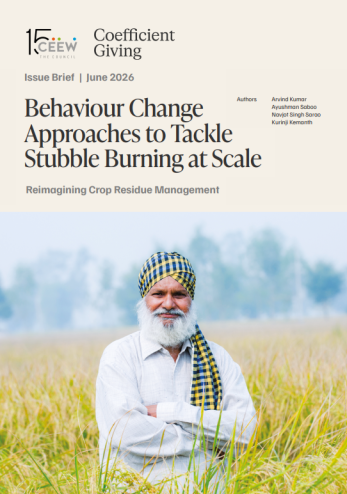
Behaviour Change Approaches to Tackle Stubble Burning at Scale
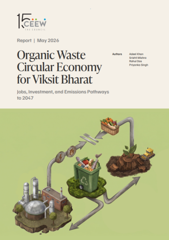
Organic Waste Circular Economy for Viksit Bharat
How Can India Tackle Air Pollution with an Airshed-level Approach?
Roadmap of the methodology to assess the climate co-benefits of the SUP ban in Tamil Nadu
Roadmap of the methodology to assess the climate co-benefits of the SUP ban in Maharashtra