Council on Energy, Environment and Water Integrated | International | Independent
Suggested citation: Mohan, Dharshan Siddarth, Sabarish Elango, Hemant Mallya, and Himani Jain. 2025. How Will India’s Vehicle Ownership Grow? A District-level Outlook to 2050. New Delhi: Council on Energy, Environment and Water (CEEW).
Disaggregated projections of vehicle population are crucial for informed policymaking and infrastructure planning at the regional level across the country to improve management of challenges like congestion and urban pollution. This report presents an estimation of the future vehicle stock (i.e., the total number of active vehicles on the road) and ownership levels (i.e., the number of vehicles per 1,000 people) at the district level for ten different vehicle categories including 2W, 3W, 4W, buses and trucks. Using historical registration data from the VAHAN portal and segment-wise survival rates, this report derives the baseline vehicle stock in the year 2023. Then, the report projects the future vehicle stock by using projections of GDP and population at the district level till the year 2050. This study highlights key regional growth patterns and emerging trends across vehicle segments.
India’s steadily growing economy, coupled with rising income levels and urbanisation, is set to further drive the expansion of its automobile industry, which is already the third largest globally (Nikkei Asia 2024). While aspirational and convenience-driven choices are fuelling the growth of personal vehicles, the increasing demand for goods vehicles is being driven by the growth in trade, industries, and e-commerce.
In this context, having detailed and disaggregated data on the number of active vehicles on road (the vehicle stock) is essential for informed policymaking and infrastructure planning, enabling better management of challenges such as congestion and urban pollution. Considering limited information on disaggregated data, our study aims to fill this void by projecting vehicle stock at the district level.
Our study estimated the vehicle stock from the year 2024 till 2050 by:
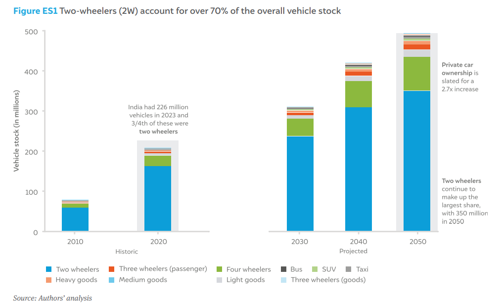
Our projections show that the total number of vehicles in the country will more than double from the 2023 level of 226 million to 494 million in 2050. Two-wheelers will continue to dominate the vehicle stock, with 350 million units in 2050 (up from 175 million in 2023). Private cars will grow by over 2.7 times, from 32 million units in 2023 to 90 million units in 2050.
The ownership levels (number of registered vehicles per unit of population) of vehicles in India will double by 2050, compared with 2023 levels. For reference, China has 310 vehicles per 1,000 people already in 2023, almost twice that of India. However, its GDP per capita is five times higher than India’s. By 2050, India’s GDP per capita (in constant prices) is projected to reach USD 10,500, a level comparable to China’s in 2024. Correspondingly, vehicle ownership in India is expected to reach 309 vehicles per 1,000 people.
Similarly, the EU28 countries have an average ownership level 3.7 times higher than India’s (~600 vehicles per 1,000 people), but with a 17 times higher GDP per capita.
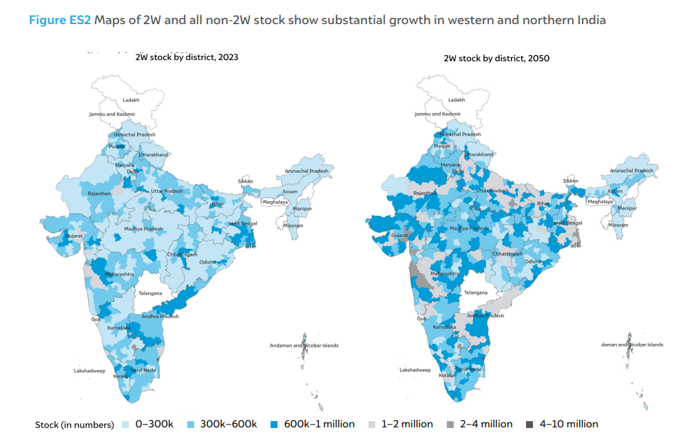
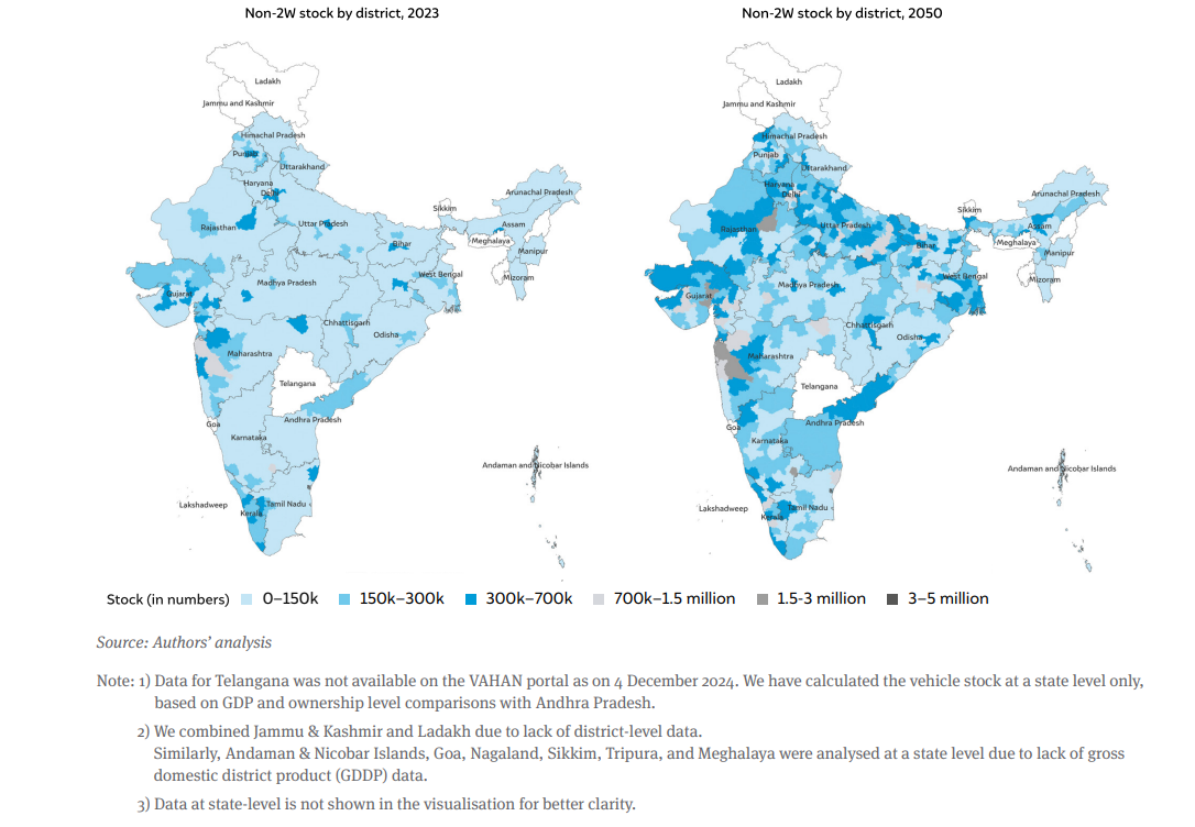
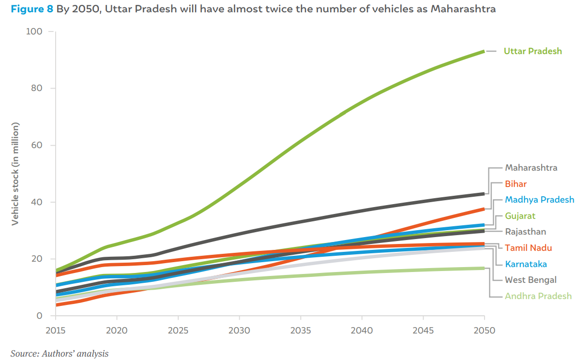
Figure ES2 shows the vehicle stock in 2023 and 2050 in a simplified district map. At the state level, we found that Uttar Pradesh will have the largest stock in 2050 by far, with more than 90 million vehicles, a bulk of which are 2W at 68 million. Similarly, Bihar will also see a substantial growth in stock, from about eight million vehicles in 2023 to 30 million by 2050. Maharashtra, Madhya Pradesh, and Gujarat will complete the top five states by stock. The southern states show a limited increase in vehicle stock; the population levels in these states start declining by 2030, thus causing a saturation in vehicle stock. States like Tamil Nadu, Kerala, Andhra Pradesh and Karnataka (except for Bengaluru district) do not show a major increase in stock.
At the district level, we found that substantial growth in stock is seen in some western districts (like Mumbai, Thane, Surat and Kachchh) and districts in northern states (like Delhi, Uttar Pradesh and Bihar). Delhi could have 10 million vehicles by 2050, doubling from about five million in 2023. In the south, growth is seen mainly in Bengaluru district, which will have the second highest stock at a district level in 2050. Thane, Pune and Ahmedabad will complete the top five districts by stock.
Of nearly 640 districts (as per the 2011 census) analysed, the top 10 districts by stock in 2050 alone account for 10 per cent of the projected national stock in 2050. This highlights the need for strong policymaking and infrastructure planning to manage and mitigate such growth, especially in metro cities and urbanising regions.
Based on the findings, we make the following recommendations:
India is one of the fastest-growing major economies, and the automotive industry is a significant contributor to its growth. With strong backward and forward linkages, liberalisation, and policy interventions, the automotive industry’s contribution to India’s GDP has risen from 3 per cent in 1992–93 to over 7 per cent today. It accounts for 12 per cent of the gross value added (GVA) in the manufacturing sector, contributing half of India’s manufacturing GDP, and employs 32 million people directly and indirectly (Cogoport 2022). India’s automobile market continues to proliferate, with domestic vehicle sales surpassing that of Japan for the first time in 2023, making it the third largest in the world (Nikkei Asia 2024).
The World Bank classifies India as a lower-middle income country (The World Bank n.d.) based on its per capita income of USD 2,484/year (as of 2023); there is immense scope for economic growth and development for the country and its citizens. Such development will continue to drive demand for automobiles with the emergence of the neo-middle class and their aspirations to own vehicles due to higher disposable incomes. India is pegging its economic growth on increased industrialisation, which will need a larger freight carrying capacity, and hence, more medium and heavy-duty vehicles. E-commerce is also picking up in India, leading to increased last-mile delivery requirements that need light duty goods vehicles.
However, growth in on-road automobiles has several negative impacts. Indian cities are already facing critical issues such as congestion and elevated levels of urban pollution. An increase in the number of vehicles on the road will significantly elevate the exposure to hazards, thereby increasing the risk to individual safety and health.
There is limited data on the number of vehicles plying on Indian roads (i.e., the vehicle stock); government data does not track the number of active vehicles. This study estimates the existing vehicle stock and potential growth trajectories over the next two and a half decades to improve data at a regional level for planning of both the supply side (automobile and component manufacturing) and demand side (fuel supply, roads and other infra). This granular data will be essential in efficient policymaking to decarbonise the vehicle fleet while meeting the population’s growth aspirations.
Previous studies that projected vehicle stock and ownership levels have used Gompertz, log-linear, and logistic functions to project vehicle ownership. Among the models listed, the Gompertz function is deemed more appropriate and better fits the historical trends than other models (Wu, Zhao and Ou 2014).
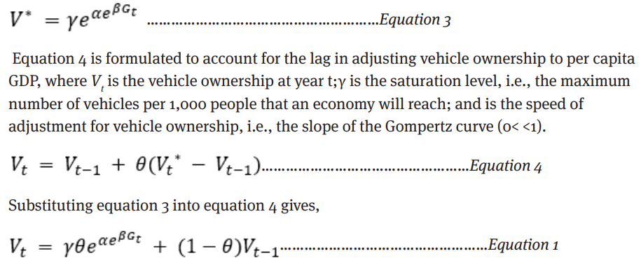
Typically, the Gompertz function has per capita GDP as a key independent variable. The country’s per capita GDP directly affects the change in vehicle ownership, depicted by an ‘S’- shaped curve or a sigmoidal curve (Arora et al. 2011). It assumes that growth will start slowly at low-income levels, then accelerate as income rises, and finally slow down as saturation approaches (Dargay et al. 2007; Wu et al. 2014). Equation 1 below provides the Gompertz function. A more detailed explanation of the function and its terms is given in Section 3.5.

Vt is the vehicle ownership at year t; is the saturation level; is the speed of adjustment; α and β are shape parameters; G denotes per-capita income. The saturation level (γ) is the maximum level of vehicle ownership (vehicles per 1,000 people) for a country, and varied methods are used to determine it. The speed of adjustment (θ) is the rate at which vehicle ownership approaches saturation (0<θ<1)
The studies involving projections for the road transport sector in India analyse vehicle stock growth by segment, using the projected values to estimate future oil demand, emissions, and energy consumption (Arora, Vyas and Johnson 2011; Singh, Mishra and Banerjee 2020). A previous CEEW study (Soman et al. 2020) developed the vehicle stock across all passenger vehicle segments at national level. However, none of these studies have attempted to project the vehicle stock at a regional level. This study aims to address this gap by providing regional-level projections of vehicle stock, allowing for more granular understanding of trends and variations in different regions.
Different studies have used different saturation levels. The level used in the Gompertz function for the UK and other industrialised economies lies between 0.4 and 0.7 (vehicle ownership per 1,000 people) (Button, Ngoe and Hine 1993). The study by Huo et al. (2007) analysed the data from 18 countries and deduced that the saturation rate for the US as a representative of North America was 0.8. Similarly, Europe’s saturation level was 0.6, and Japan’s, as a representative of Asian economies, was 0.55.
For India, the study by Singh, Mishra and Banerjee (2020) examined the growth of twowheelers (2W) and cars individually under two distinct scenarios: conservative and aggressive. They have set the saturation levels at 0.25 and 0.35 for 2W and 0.15 and 0.25 for cars, respectively, in each scenario. The CEEW study (Soman et al. 2020) divided the vehicle stock into 2W and combined all other vehicle categories (as the combined saturation level for the latter is still much lower than that of 2W). They have assumed the saturation level to be 0.25 for 2W and 0.15 for all other vehicles combined. The Indian studies assumed saturation levels based on trends observed in other countries like China and Japan.
From the literature review, we found that all prior studies used pre-determined saturation levels that the countries could eventually reach. De Silva et al. (2022) hypothesised that countries could have varying saturation levels, and that it would not be a universal constant. The saturation level (γ) is influenced by many variables such as infrastructure, household size, population density, and share of public transport. Considering India’s regional diversity in culture, income levels, infrastructure, etc., the use of γ as a near-constant value across districts and states may not be appropriate. Thus, using geography-specific γ will provide a clearer picture of vehicle ownership estimates, allowing for more complex policy variable interactions.
In this context, our current study estimates vehicle ownership at district level in India for 2050, building upon the CEEW 2020 study and its approach. It delves into more detail, examining the heterogeneity in vehicle ownership patterns across individual states and districts which allows us to discern regional disparities and trends. We use district-specific saturation rate (γ) and speed of adjustment (θ) (see Section 3.5) to estimate the district-level vehicle stock and its growth, aiding sub-national level policymaking.
Our vehicle stock projections followed a multi-step calculation process, starting with estimating the historical stock of vehicles on the road every past year. We used historical vehicle registrations data to calibrate the Gompertz function (using historical GDP and population data) through minimising the sum of errors squared between the actual values and calculated values, i.e., by matching calculated values with the actual historical data by varying γ and θ. We then applied the Gompertz function at a district level to project future vehicle ownership and stock based on projected district-level GDP and population data. The forthcoming sections explain the specific methods and assumptions in more detail.
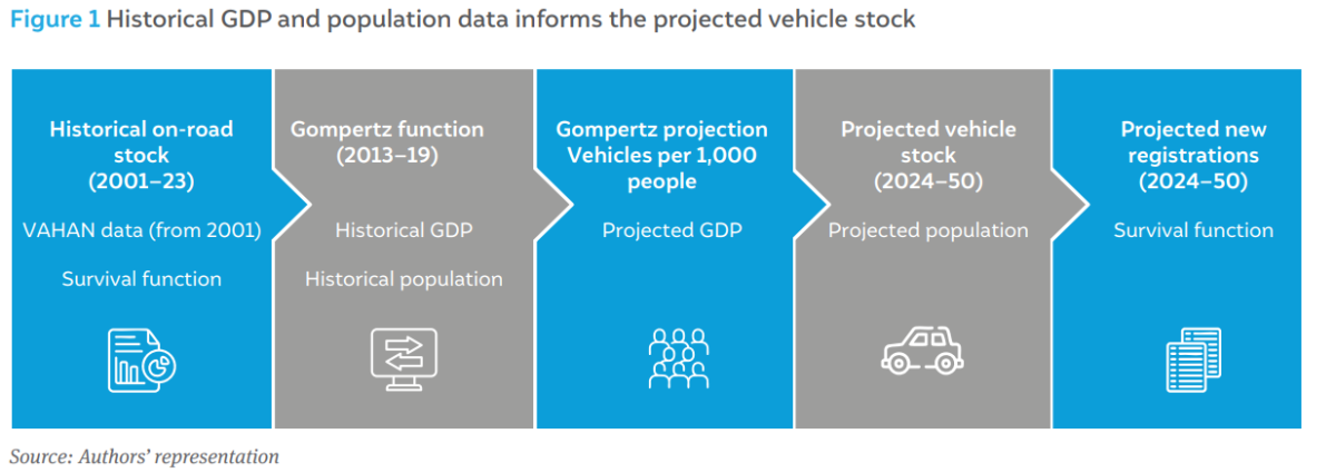
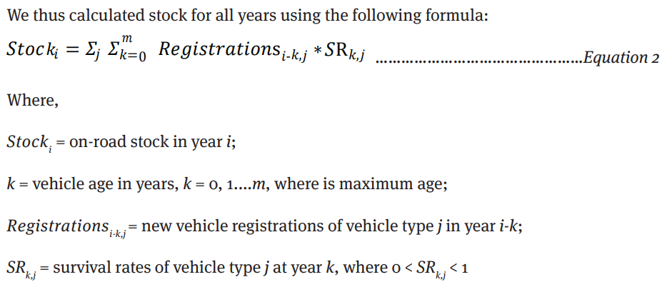
Establishing historical stock is a prerequisite for estimating future stock projections. The first step in estimating vehicle stock at a regional level was to compile data on the number of registered vehicles each year. Then, we estimated the stock in year ‘y’ by adding the new registered vehicles at year ‘y’ and the legacy vehicles that have survived until the year ‘y’. We used this method to calculate annual stock by vehicle segment from 2001 to 2023. This analysis uses 2001 as the base year, before which no data was publicly available at the regional level. Therefore, we do not consider any active vehicles registered pre-2001. This is not a significant issue because almost 99 per cent of these vehicles are out of service and not a part of active stock by 2015. Hence, although our stocks are an underestimation till 2015, the forecast itself begins in 2023, by which time all the pre-2001 vehicles will have been out of active service.
We utilised the VAHAN dashboard (Ministry of Road Transport and Highways 2024) to extract data on the segment-wise annual registrations at a regional transport office (RTO) level between 2001 and 2023. We then aggregated all the RTOs to the district level (as per the 2011 Census), as other data such as GDP and population are available at a district level only. Across different states, RTOs have different jurisdictions and hierarchies; thus, the jurisdiction boundaries from the respective state transport department websites were collected. We mapped the RTOs to each district except for Delhi, where several RTOs have jurisdiction over smaller areas that are not mainly linked to any district or sub-district boundary. For Delhi, we have combined all its districts to represent it as one district in our study, as it is a small region.
Using the annual registration data at a district level, we then arrived at the total number of active vehicles by considering ‘survival rates’ for different vehicle categories. These survival rates predict the number of vehicles of a given category that will go out of service after each year. Survival rates are critical for calculating vehicle stock, as registration data alone does not account for vehicles that go out of active service or are scrapped (since the road transport department does not yet mandate a vehicle de-registration process). Section 3.2 has more information on survival rates and their calculation.
Table 1 Classification of vehicle categories as adapted from the VAHAN dashboard
| Vehicle category | Vehicle class as per VAHAN | Remarks |
|---|---|---|
| 2W | Adapted vehicle; M-Cycle/Scooter; M-Cycle/ Scooter with side car; Moped; Motor cycle/ Scooter used for hire; Motor cycle/Scooter with trailer | Of all the given categories, M-Cycle/Scooter is the predominant one by number of registrations; the other categories were subsumed under 2W for completeness. |
| 3W-Passenger (3W-P) | Three-wheeler (Passenger); Three-wheeler (Personal) | |
| 3W-Goods (3W-G) | Three-wheeler (Goods) | |
| 4W private (hatch/ sedan) | Motor Car | The VAHAN dashboard does not differentiate between hatchbacks/sedans and SUVs. However, the GST Council defines SUVs as a separate category that attracts higher GST rates. We therefore split the registrations under the ‘Motor Car’ category into hatch/sedan and SUV based on the model-wise and region-wise sales data reported by the Society of Indian Automobile Manufacturers (SIAM) (2023a; 2023b). According to SIAM, SUVs are classified under utility vehicles (UVs) category. While historical data on UVs was available from SIAM, specific data on the share of SUVs within UVs was available only for the year 2023. Consequently, this share was assumed to remain constant for the prior years. |
| 4W private (SUV) | Motor Car | |
| Taxi | Luxury Cab, Maxi Cab, Motor Cab | The given taxi categories in VAHAN do not differentiate between hatchbacks and SUVs. For the sake of simplicity, we assumed that all vehicles under this category are hatchbacks/sedans. |
| Bus | Bus, Educational Institution Bus, Omni Bus, Omni Bus (Private Use) | We did not differentiate buses into any size categories (such as 9 m, 12 m, etc.) as VAHAN does not provide any such split. |
| Light Goods Vehicle (LGV) | Goods Carrier (Light Goods Vehicle) | Goods vehicles with a gross weight of less than 7.5 tonnes |
| Medium Goods Vehicle (MGV) | Goods Carrier (Medium Goods Vehicle) | Goods vehicles with a gross weight of between 7.5 and 12 tonnes |
| Heavy Goods Vehicle (HGV) | Goods Carrier (Heavy Goods Vehicle) | Goods vehicles with a gross weight of over 12 tonnes |
Source: Authors’ compilation
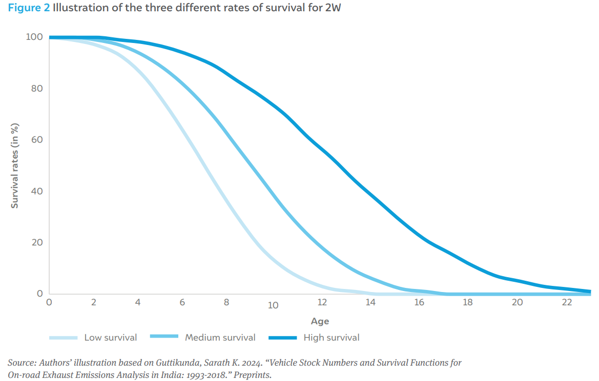
Survival rates are used to translate cumulative annual vehicle registrations into vehicle stock. A study by (Pandey and Venkataraman 2014) used a logistic function to establish survival rates, whereas (Goel, Guttikunda, et al. 2015) utilised a probabilistic Weibull distribution, denoting the probability of a vehicle’s use after a certain number of years (Zachariadis, Samaras and Zierock 1995, Baidya and Borken-Kleefeld 2009, Goel, Guttikunda, et al. 2015, Goel, Mohan, et al. 2016). For this analysis, we have chosen the latter because it provides three distinct scenarios for estimating survival rates. Moreover, the shape parameters derived by (Guttikunda 2024) are based on multiple fuel station surveys conducted in different cities and are much more recent (Goel, Guttikunda, et al. 2015, Goel, Mohan, et al. 2016, BSPCB 2019).
Figure 2 summarises the survival rate for a typical two-wheeler for three scenarios: low, medium, and high survival rates. We classified regions into tiers as per the Reserve Bank of India’s classification system (Reserve Bank of India 2016). We mapped Tier-1 cities like Chennai, Mumbai, Delhi, and Kolkata to lower survival rates, meaning vehicle turnover is the highest in such cities. Similarly, we mapped Tier-2 cities like Coimbatore, Indore, Kanpur, and Kochi to medium survival rates and Tier-3 (and higher) locations to high survival rates.
Due to the delayed decadal census exercise, we were unable to establish district-level population growth trends using historical census data. A 2019 report from the Ministry of Health and Family Welfare (MoHFW) provides state-level population projections until 2036 (National Commission on Population 2019). It also provides expected urban vs rural population growths in each state. We used this data to prepare district-level population projections. For all years beyond 2036, we extrapolated the growth trends observed in the MoHFW data such that the state-level population projections merged in our populationpeaking estimations by CEEW. Based on CEEW assumptions, the country’s population growth will slow towards 2050 and peak by 2060.
Historical data on Gross state domestic products (GSDPs) are available with the RBI. We projected these GSDPs for different states based on the expected levels of growth of the national Gross domestic product (GDP) by 2047; we assumed that states with lower Gross domestic product (GDP) in the present year would grow faster than the national average growth rate than states with higher GSDPs.
However, there is no central agency that maintains historical data on Gross district domestic product (GDDP). Some state government departments have published their respective GDDP data for two to three recent years. However, the data is not consistently available. Table 2 shows the extent of consistent GDDP data availability for each state.
Table 2 Inconsistent availability of latest GDDP data poses a challenge for more accurate projections
| State | Availability year | State | Availability year |
|---|---|---|---|
| Andhra Pradesh | 2019–20 | Haryana | 2004–05 |
| Arunachal Pradesh | 2019–20 | Himachal Pradesh | 2004–05 |
| Karnataka | 2019–20 | Jharkhand | 2004–05 |
| Maharashtra | 2019–20 | Madhya Pradesh | 2004–05 |
| Puducherry | 2019–20 | Manipur | 2004–05 |
| Tamil Nadu | 2019–20 | Mizoram | 2004–05 |
| Uttarakhand | 2019–20 | Punjab | 2004–05 |
| Uttar Pradesh | 2019–20 | Andaman & Nicobar Islands | Not available |
| Assam | 2009–10 | Delhi | Not available |
| Bihar | 2009–10 | Goa | Not available |
| Kerala | 2009–10 | Gujarat | Not available |
| Odisha | 2009–10 | Jammu & Kashmir | Not available |
| Rajasthan | 2009–10 | Meghalaya | Not available |
| Telangana | 2009–10 | Nagaland | Not available |
| West Bengal | 2009–10 | Sikkim | Not available |
| Chhattisgarh | 2004–05 | Tripura | Not available |
Source: Authors’ compilation from state government reports
We collected all the available historical data and calculated GDDP per capita in the year for which data was available, using the respective district-level population. We then found the ratio of GDDP per capita to GSDP per capita for that year; all future years’ projections used this ratio multiplied by the projected GSDP and population to partially account for the mismatched base years (assuming that population is somewhat correlated to GDP). Because the population projections use different growth rates for urban and rural population in each district, the GDDP shares of all districts in a state will change year-on-year, based on the changing population share of the districts.
For those states/UTs with no data, we only made state-level stock projections. These include the Andaman and Nicobar Islands, Jammu and Kashmir, Delhi, Goa, Sikkim, Nagaland, Tripura, and Meghalaya. Gujarat is the only exception, for which we assumed the GDDP per capita distribution to be similar to Tamil Nadu (as the latter has a similar GSDP). The Annexure contains our estimates of district-level GDDP per capita.
We employed the Gompertz function to estimate India’s future vehicle ownership until 2050. The function used is assumed from Dargay, Gately and Sommer (2007), where V* represents the long-run equilibrium level of vehicle ownership, and G signifies per capita GDP. The γ is the saturation level (in vehicles per 1,000 people), and ɑ and ß are negative parameters that determine the shape of the curve.
The significant parameters affecting the equation are saturation level (γ), speed of adjustment (θ), GDP (per capita income), and ɑ and ß (shape parameter constants). In our analysis, we identified the saturation level and speed of adjustment for each district and vehicle category listed in Table 1. To achieve this, we calibrated the Gompertz parameters for each district by minimising the sum of errors squared (known as ‘least squares method’), with the historical growth in ownership levels.
We attempted the calibration of the Gompertz curves (by changing the saturation level and speed of adjustment) at a state level using four sets of historical stock data: 2011–2019, 2011–2022, 2013–2019, and 2013–2022. We chose the 2013–2019 scenario as the projections more closely matched the actual data for more than 70 per cent of states and vehicle categories (i.e., the sum of the squared differences between actual vs calculated data was lowest below 10 per cent). Using this scenario, we repeated the calibration process for each vehicle category in every district, allowing us to determine the saturation levels and speed of adjustment based on historical patterns and growth rates observed in each district.
We then substituted the values of saturation and speed of adjustment in Equation 4 to determine the ownership levels until 2050 for each district and vehicle segment. The ownership level (in vehicle units per 1,000 people) is then converted to stock using the district’s projected population data. The last step is to back-calculate the annual new registrations using the survival rates to match the projected stock from Equation 1.
The vehicle stock projection and subsequent new vehicle registration estimates are based on the aforementioned data and assumptions. This section discusses the results of vehicle stock projection and ownership levels by segment at the regional and national level. We then go on to compare our national stock estimates with existing transportation stock forecast models.
We projected the vehicle ownership by segment and district from 2024 to 2050 using Equation 4. We then calculated the national-level estimates by aggregating at the district and state level.
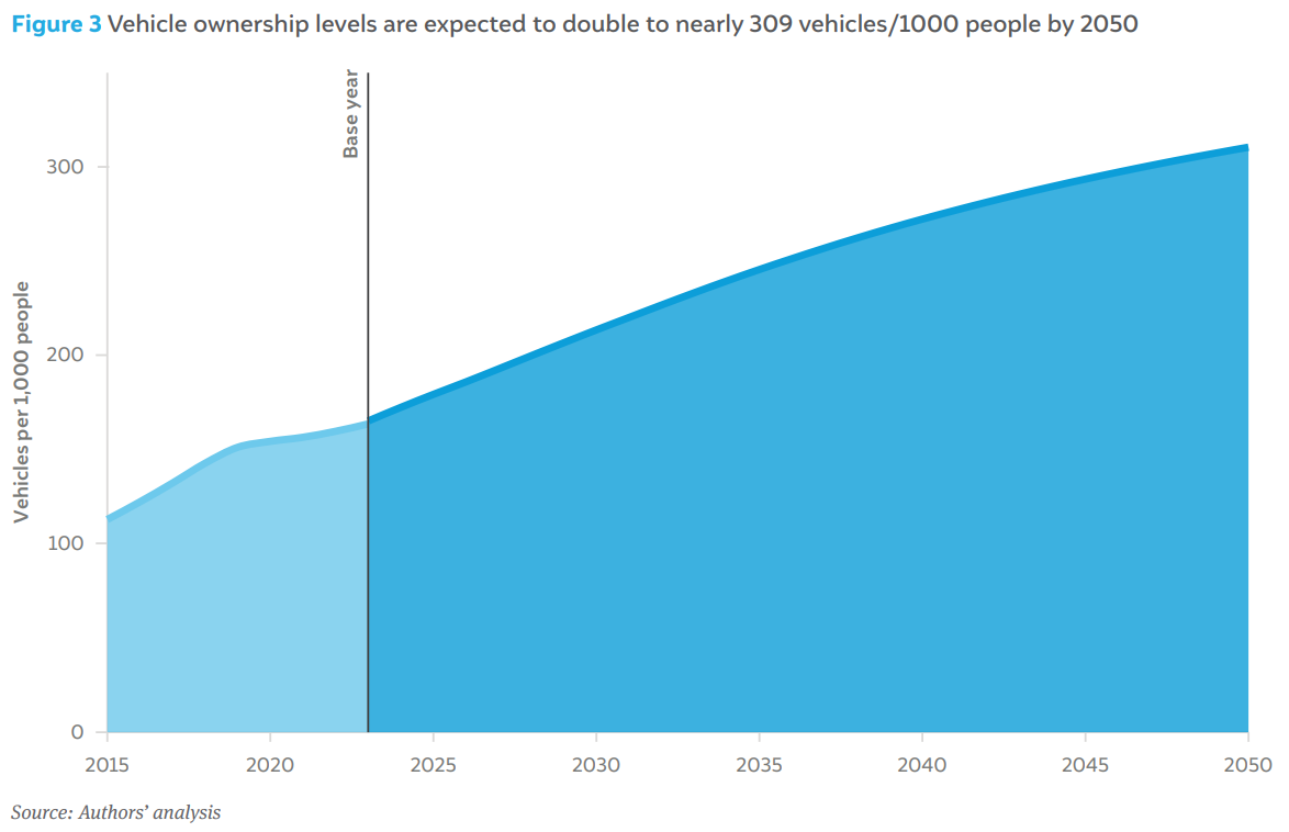
We estimate that the total vehicle ownership (inclusive of all segments mentioned in Table 1) will reach 309 per 1000 people in 2050, compared to 163 per 1000 people in 2023, as observed in Figure 3. The slight change in trajectory observed between 2019 and 2022 is caused by the COVID-19 pandemic, when actual new registrations were at an all-time low, significantly impacting the stock and, subsequently, the ownership levels. In comparison, China had approximately 310 vehicles per 1,000 people in 2023, while the European Union countries had an average of nearly 600 vehicles per 1000 people (Xinhua News Agency 2024, Eurostat 2024). Interestingly, the GDP per capita of China (at USD 12,970 in 2024) is around five times higher than that of India (at USD 2,700), while that of the EU (at USD 46,640) is 17 times higher (International Monetary Fund 2024). However, the vehicle ownership in China and the EU are only 2 and 3.7 times higher respectively, as these regions are more urbanised and have much bigger public transport systems.
By 2050, India’s GDP per capita (in constant prices) is projected to reach USD 10,500, a level comparable to China’s in 2024. Correspondingly, vehicle ownership in India is expected to reach a similar level to China’s current ownership level.
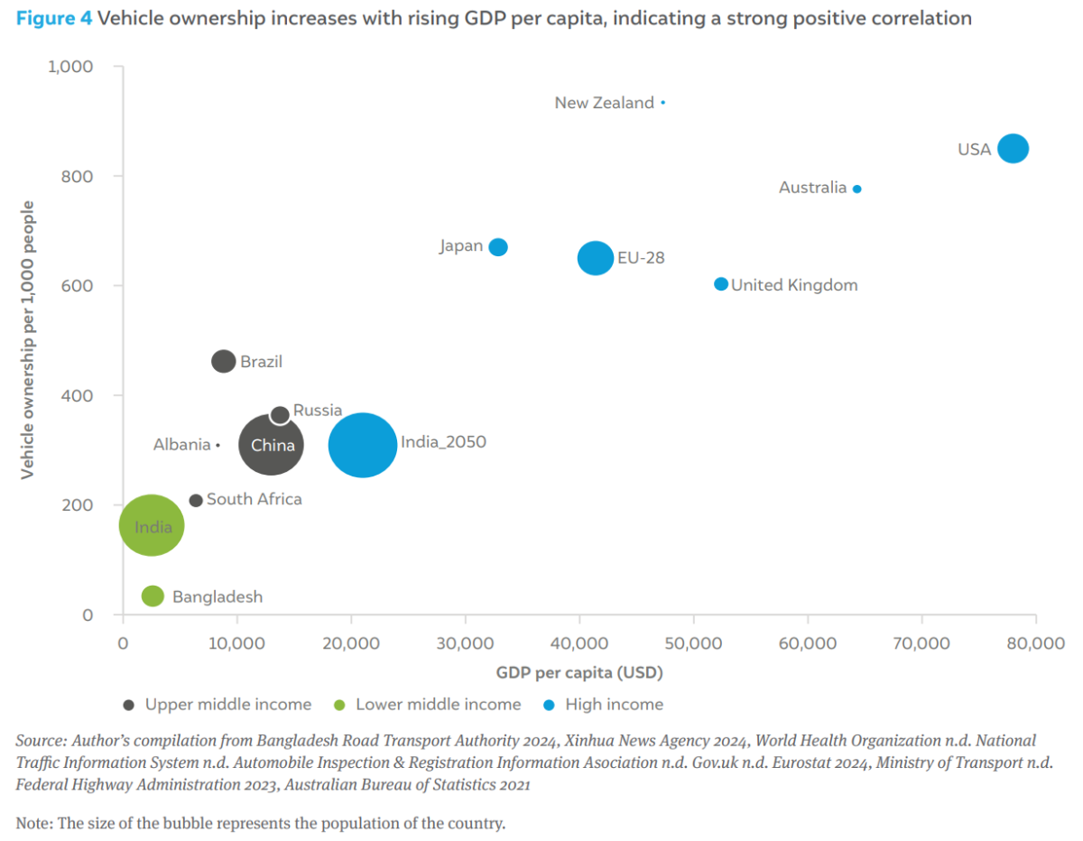
Figure 4 illustrates the relationship between vehicle ownership and GDP per capita across various countries, categorised by income group based on the World Bank classification (The World Bank n.d.). Among the listed nations, New Zealand records the highest vehicle ownership, with 934 vehicles per 1,000 people and a GDP per capita of approximately USD 47,000. We attribute this high ownership level to the country’s low population density and dispersed housing patterns, making vehicles essential for mobility. The USA is next, with 850 vehicles per 1,000 people and a GDP per capita of approximately USD 78,000. A relative lack of public transport and car-centric urban planning contributes to the high rate of vehicle ownership in that country. Australia, the European Union (EU-28), and Japan also rank among the top five, exhibiting high vehicle ownership due to similar urban development patterns and economic conditions.
In contrast, China, Russia, and South Africa, categorised as middle-income countries, have ownership rates ranging between 200 and 350 vehicles per 1,000 people. However, Brazil stands out within this group with close to 460 vehicles per 1000 people due to favourable government policies and incentives promoting vehicle ownership.
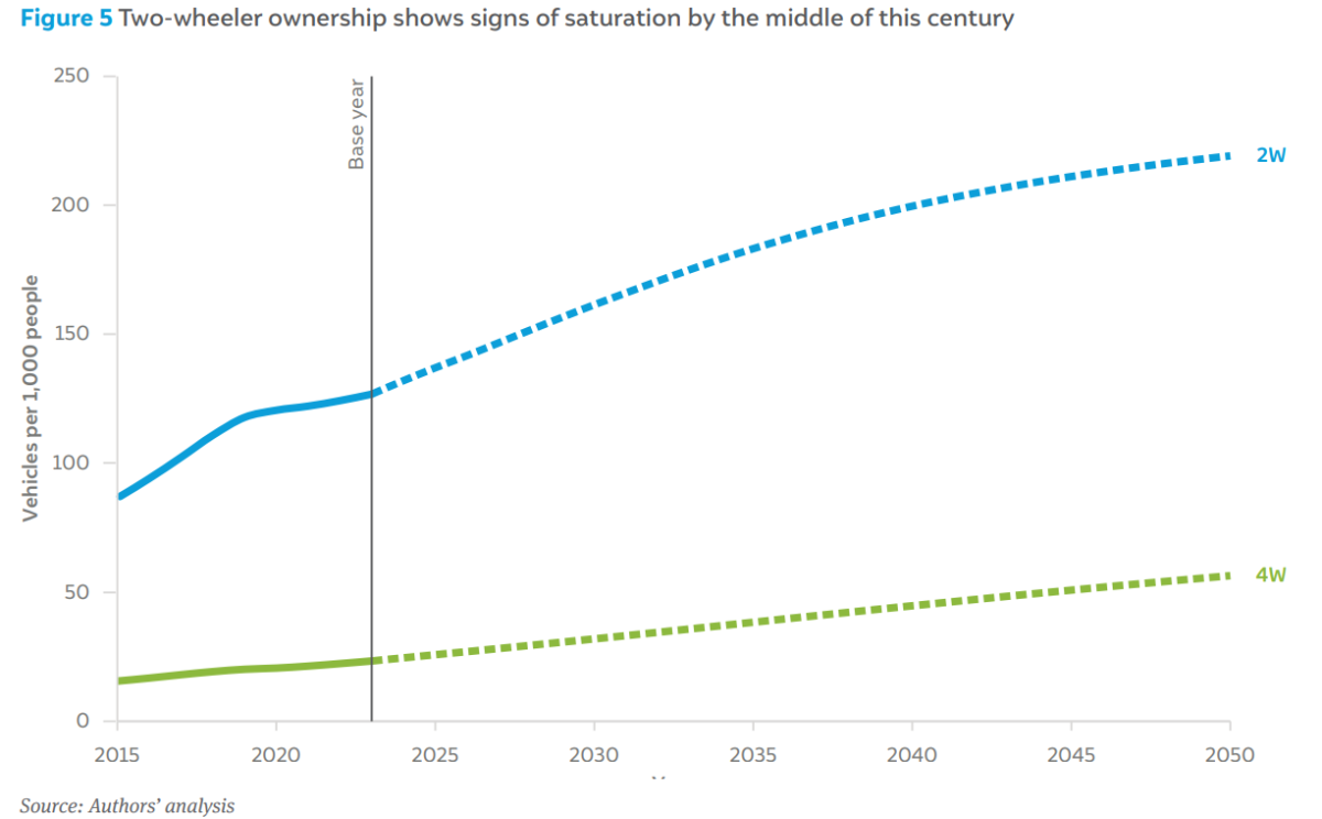
By 2050, two-wheelers are expected to account for approximately 71 per cent of the total vehicle ownership, translating to 219 2W per 1,000 people out of a total of 309 vehicle per 1,000 people. In comparison, 2W ownership in 2023 stood at around 127 per 1,000 people. While the absolute number of 2W increases by 73 per cent, their share in the overall vehicle mix declines from over 78 per cent in 2023 to 71 per cent in 2050.
Our analysis indicates that private cars (4W and SUVs) drive the overall vehicular growth, growing from 24 cars per 1,000 people in 2023 to 57 cars per 1,000 people in 2050. Even by 2050, car ownership in India is projected to be significantly lower than the 2017 levels of China, with 105 cars per 1,000 people, and Colombia, with 65.5 cars per 1,000 people (Helgi Library n.d.).
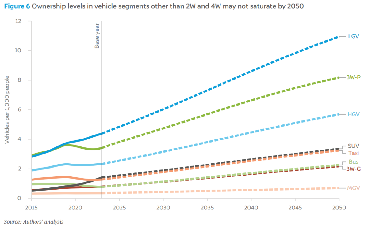
Figure 6 illustrates ownership levels of other vehicle categories (except for 2W and 4W). Other growth drivers include passenger three-wheelers (3W-P) and light goods vehicles (LGV). The number of passenger three-wheelers is projected to increase from 3.4 per 1,000 people in 2023 to 8.2 per 1,000 in 2050. Similarly, the number of LGVs is expected to rise from 4.4 per 1,000 people in 2023 to 11 per 1,000 in 2050. The number of buses per 1,000 people is low at 0.8 in 2023 but it is projected to increase modestly to 2.3 per 1,000 people in 2050. The other vehicle categories, including taxi, HGV, MGV, and 3W-G, are at the lower spectrum of the S-shaped curve, which means they might take longer to saturate.
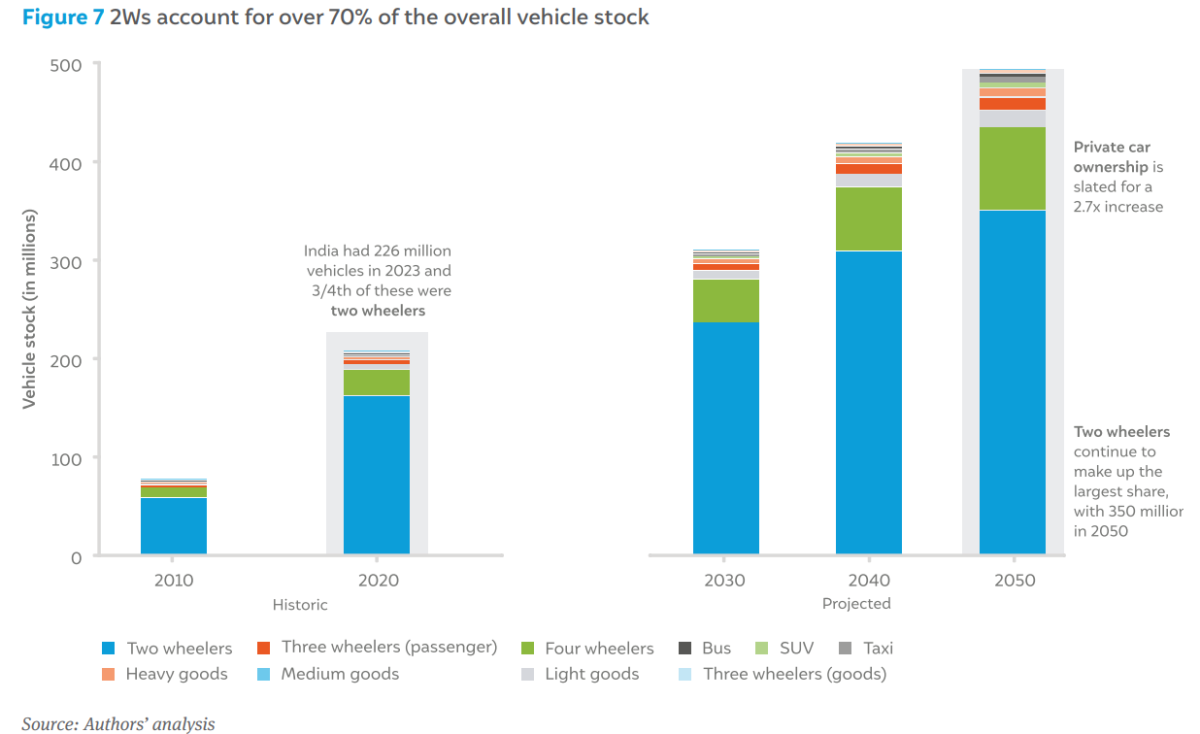
The overall stock was estimated to be at 226 million by 2023 and is projected to increase to 494 million by 2050, thus growing by nearly 2.2 times between 2023 and 2050. We estimated the total 2W on-road to be 350 million by 2050, doubling from 175 million in 2023, and forming 70 per cent of the total stock even in 2050.
Unless there is a significant upward mobility in per capita incomes, substantial increases in road infrastructure and lower taxes on 4W (currently 28 per cent for 2W and going as high as 50 per cent for SUV), we do not expect 4W to gain much share. The 4W stock will grow from 30.5 million units in 2023 (13 per cent share) to 84.9 million in 2050 (17 per cent share). Similarly, the SUV stock grows by 2.7x between 2023 and 2050, buses by 3.3x, taxis by 2.9x, LGV by 1.9x, HGV by 1.8x, and 3W-P by 1.8x.
Our analysis estimates that, by 2050, Uttar Pradesh will be the top state in terms of overall vehicle stock, followed by Maharashtra, Bihar, Madhya Pradesh, and Gujarat. Uttar Pradesh and Bihar, collectively home to approximately 27 per cent of India’s population (in 2024), are also among the poorer states in the country. With large population bases and low income levels in these states at present, we anticipate substantial growth potential in terms of per capita incomes. These two states combined will account for 25 per cent of India’s total vehicle stock in 2050. Uttar Pradesh’s stock, in particular, will grow from 29 million vehicles (in 2023) to 93 million vehicles by 2050, a threefold increase.
Among the top ten states by absolute vehicle stock, Gujarat is projected to have the highest vehicle ownership in 2050, with 351 per 1,000 people. Uttar Pradesh, Karnataka, Tamil Nadu, and Andhra Pradesh follow, with ownership levels of 336, 332, 328, and 305 vehicles per 1,000 people, respectively. Notably, while Tamil Nadu’s ownership increases by 86 vehicles per 1,000 people between 2023 and 2050, Uttar Pradesh experiences a higher increase of 214 vehicles per 1,000 people—2.5 times that of Tamil Nadu. Andhra Pradesh, Karnataka, and Maharashtra each see an increase of approximately 120 vehicles per 1,000 people, while Gujarat records a rise of 139 vehicles per 1,000 people. Meanwhile, Bihar and Madhya Pradesh witness a steep rise of 156 vehicles per 1,000 people, and 158 vehicles per 1,000 people, respectively. This trend suggests that states with lower current income levels are expected to experience more rapid growth in vehicle ownership, whereas relatively wealthier states are projected to see moderate growth in vehicle ownership.
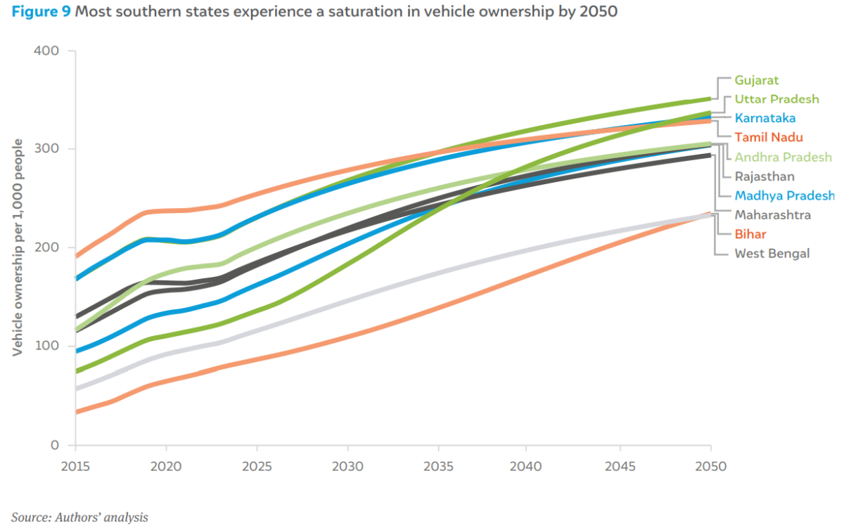
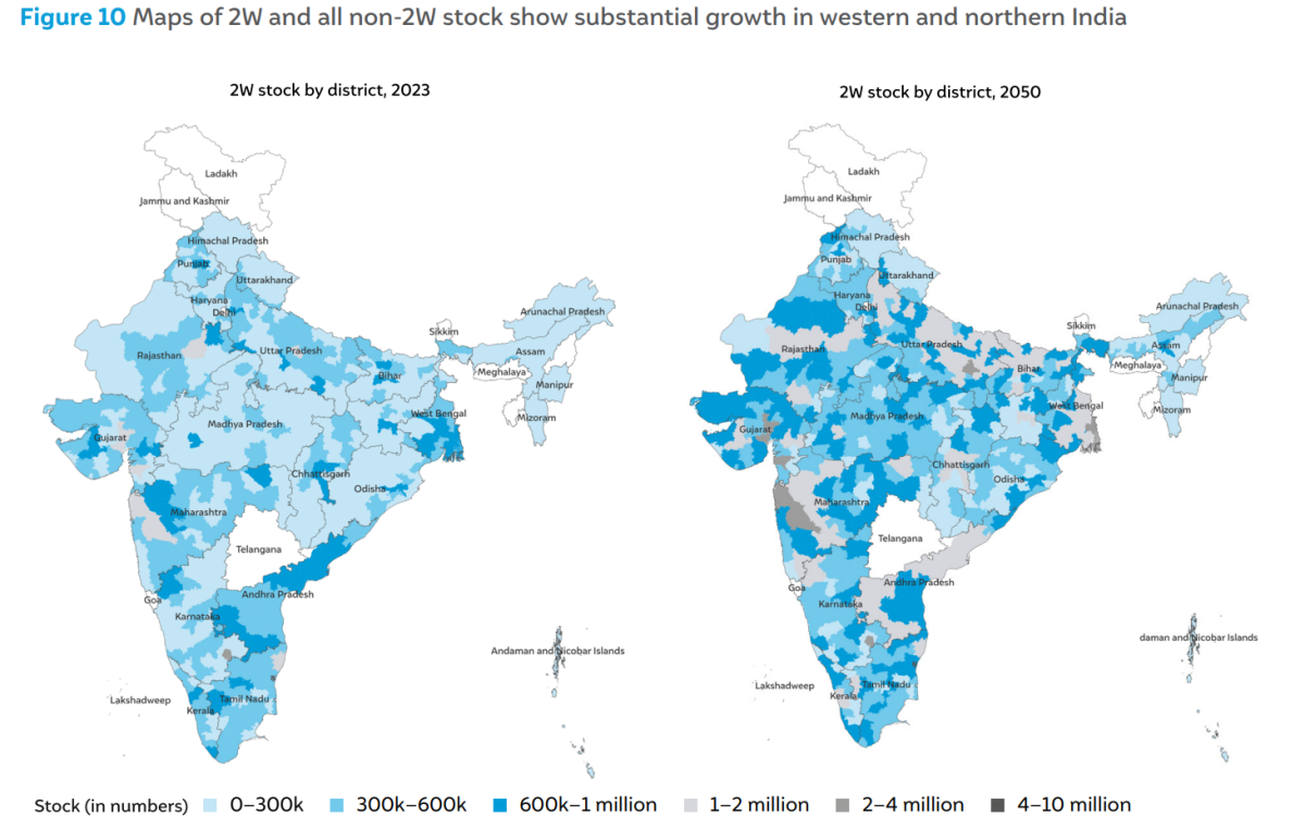
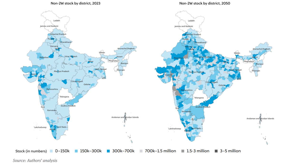
Figure 10 shows the total vehicle stock of the country on a simplified district map, splitting 2W and all other vehicles. Between 2023 and 2050, the growth in vehicle stock can be primarily attributed to the states of Maharashtra, Gujarat, Delhi, Uttar Pradesh and Bihar. Interestingly, the growth in non-2W stock is lesser in states like Uttar Pradesh, Bihar, and West Bengal compared to the 2W growth; this is likely due to the lower GDP per capita levels in these states, indicated in a preference for cheaper modes of road transport. Overall, the southern states do not show a marked increase in stock as observed in northern states, apart from some urban centres like Mumbai and Bengaluru. Southern states are experiencing population peaking in the coming decade and rising income levels; the vehicle stock thus stabilises in the near future.
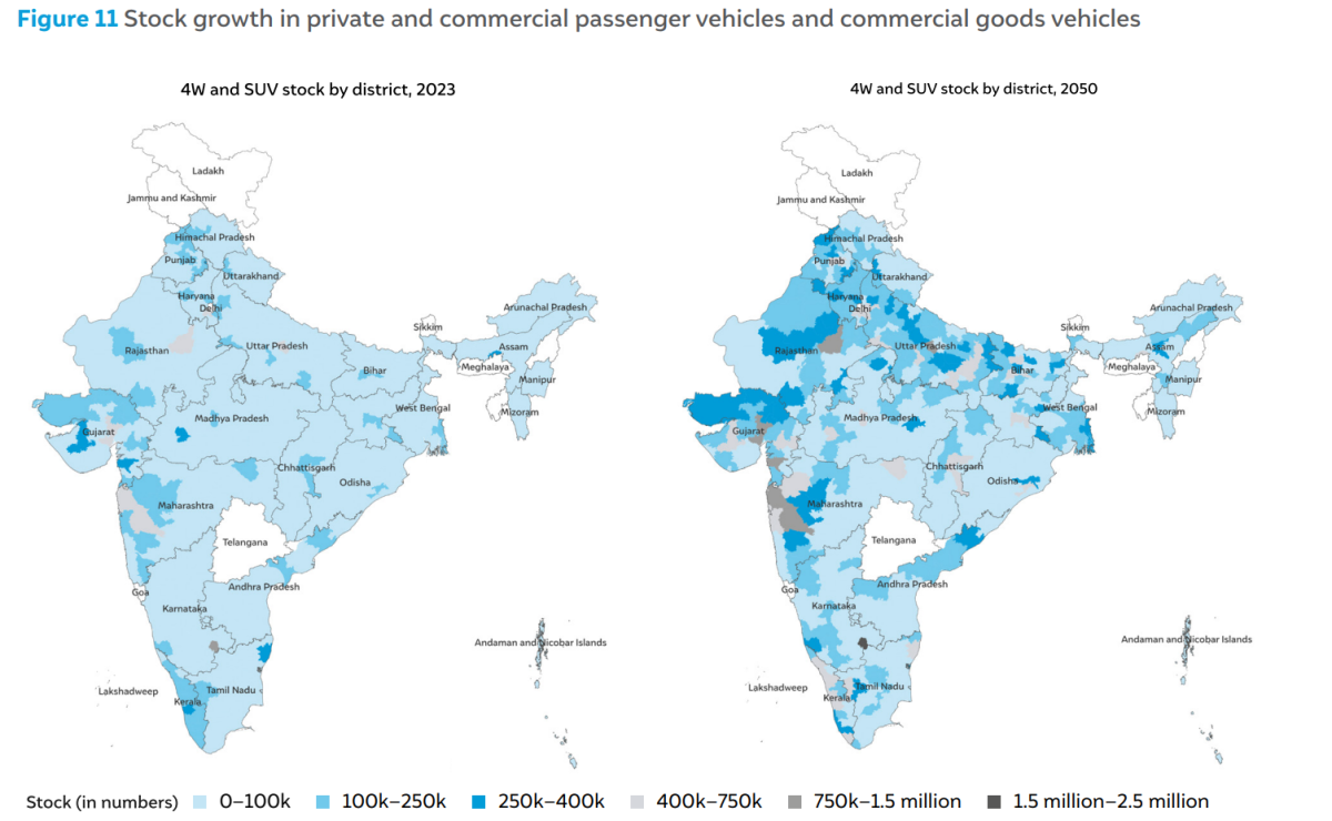
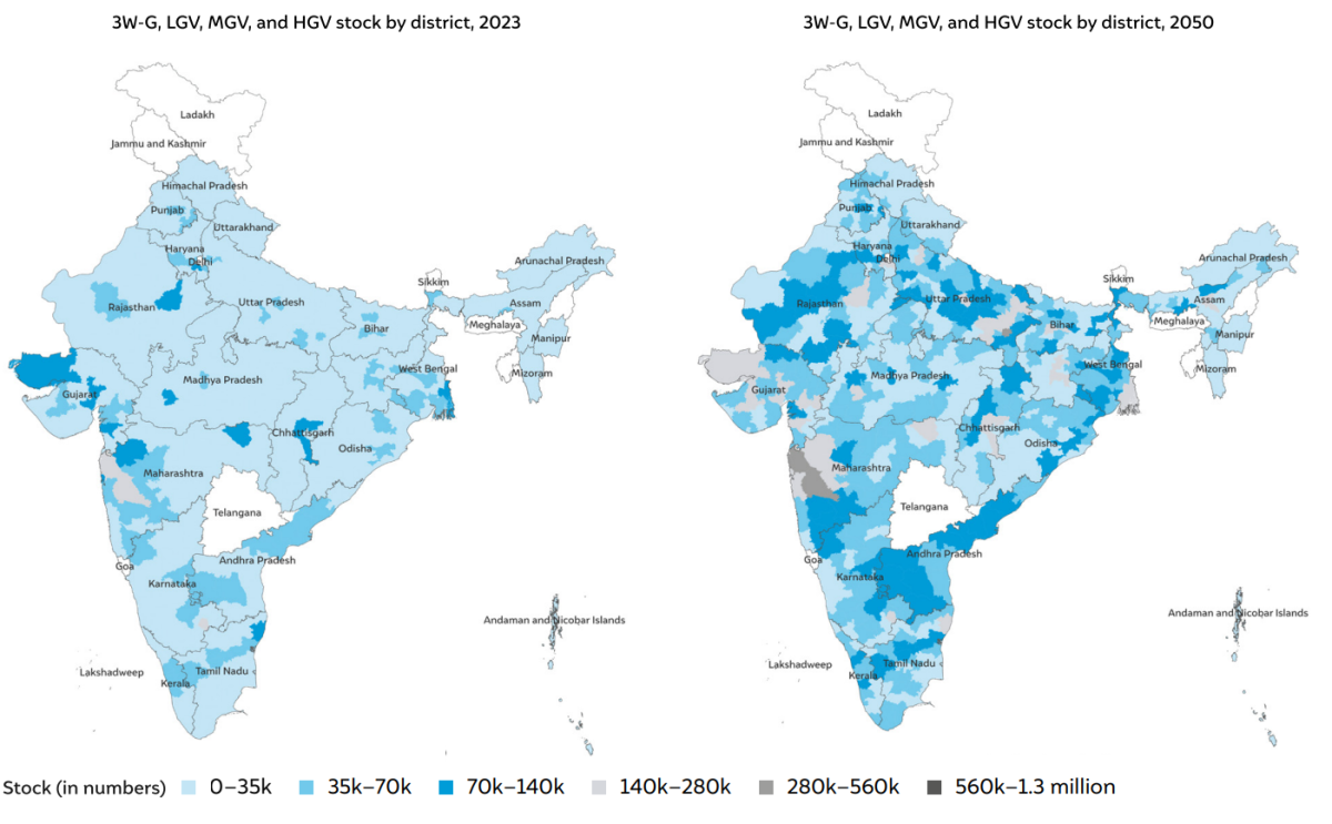
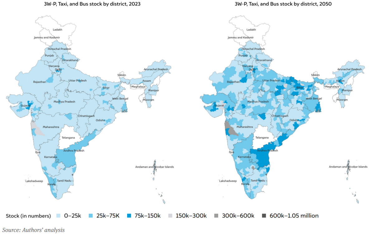
Figure 11 shows the district-level distribution of vehicle stock seen in Figure 8 at three aggregated levels: private cars (4W and SUV), public transport (3W-P, Taxi and Bus), and goods vehicles (3W-G, LGV, MGV, and HGV). Contrasting the 2W stock in Figure 10 with the private car stock in Figure 11 shows similar patterns of adoption in high-income regions; lower-income regions see lower adoption of cars than 2Ws. Public transport growth is also observed mainly in highly dense urban agglomerations like Delhi, Mumbai, Thane, Bengaluru, Ahmedabad, etc. The trends observed in new registrations over the past ten years indicate that there will be a limited role for public transport in tier-3 towns and rural areas. The projections indicate that there will be an increase in demand for goods transportation across the country, somewhat in contrast to the trends seen in private and public transport. The prevalence of goods vehicles is observed in districts that have major ports, such as in Kachchh, Surat, Mumbai, Chennai, etc. Notably, the state of Nagaland shows a notable increase in the number of goods vehicles; this is due to the large number of goods vehicles that are getting registered in the state due to tax and other regulatory benefits.
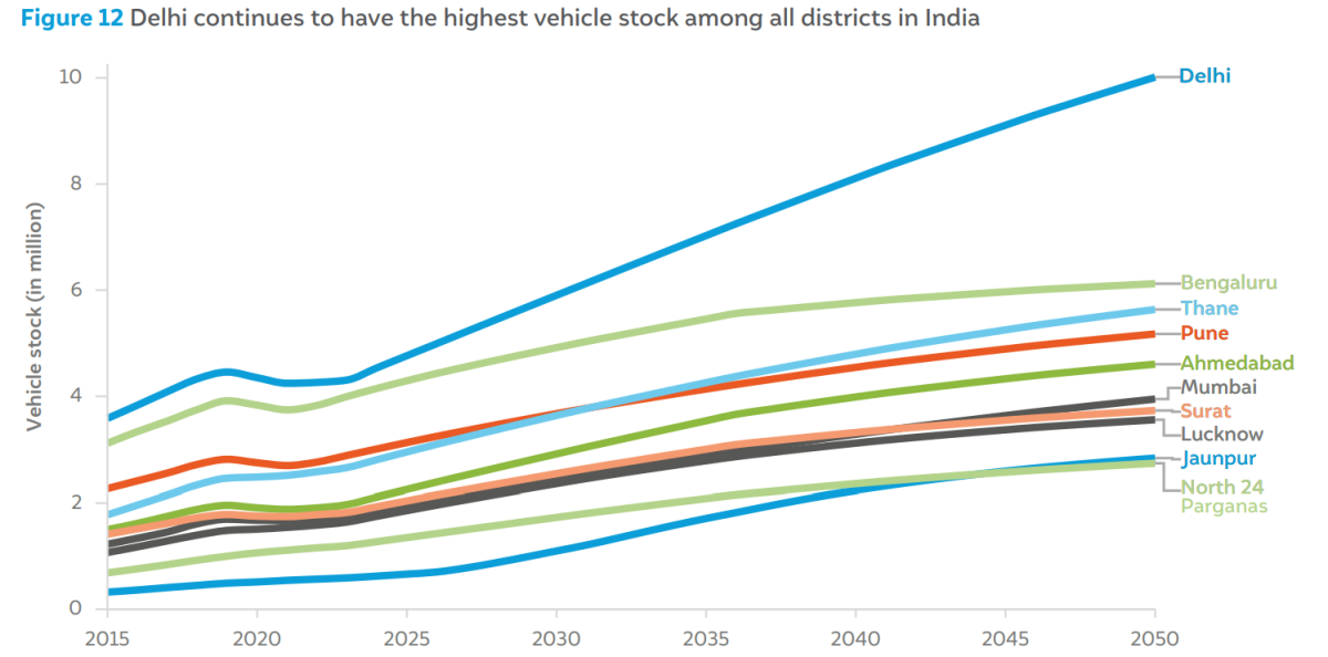
Figure 12 shows the top ten districts by vehicle stock in 2050. These 10 districts alone (out of 640 districts as per the 2011 census) account for over 10 per cent of the total national stock in 2050. The National Capital Territory of Delhi (represented as a single district) has the highest number of active vehicles, growing from 4.3 million in 2023 to 10 million in 2050. Bengaluru district in the state of Karnataka will have the second highest stock, growing from 4.0 million in 2023 to 6.1 million in 2050. The state of Maharashtra has three districts in the top ten— Thane, Pune, and Mumbai—totalling 15 million vehicles in 2050 (up from 7.2 million in 2023). The stock growth rates for almost all the top ten districts fall substantially over the years; the compound annual growth rate (average for the top ten) of 4.3 per cent from 2020–2030 reduces to 3.3 per cent from 2030–2040 and then drops to 1.7 per cent from 2040–2050. This signifies that the stock growth approaches saturation around the year 2050.
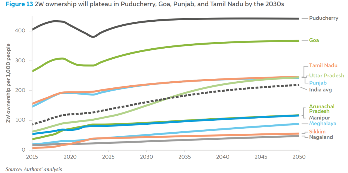
The states with the highest and lowest 2W ownership levels are shown in Figure 13. Puducherry and Goa, both coastal regions with high tourist footfall, also have the highest penetration of two-wheelers. Puducherry has over 400 2W per 1,000 people already by 2025, much higher than the national average of 150 (in 2023) or even 230 (in 2050). The states of Telangana, Punjab, and Tamil Nadu complete the top five. Apart from Uttar Pradesh, the other states start saturating in ownership due to plateauing/falling population levels towards 2050. The northeastern states of Manipur, Arunachal Pradesh, Meghalaya, Sikkim, and Nagaland have the lowest penetration of 2W; the challenging weather and terrain in these regions are the likely reasons.
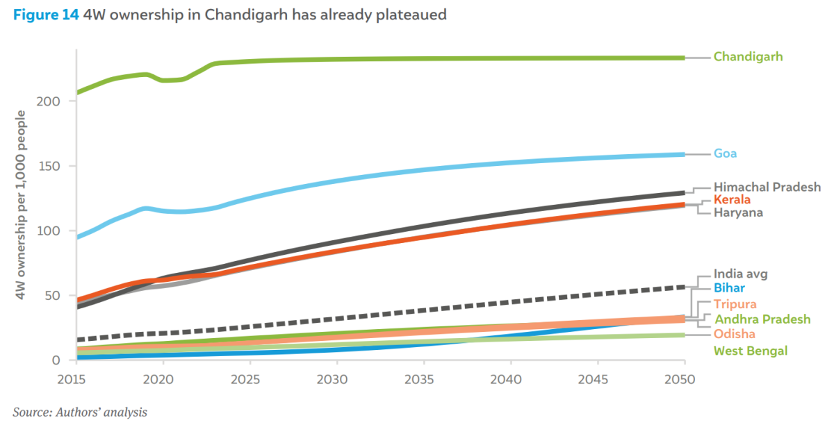
Figure 14 shows the states with the highest and lowest penetration of private four-wheelers. Chandigarh already has a much higher vehicle ownership level, potentially due to its wide roads, ample parking, and higher income levels. Himachal Pradesh is among the top ten states in terms of per capita income and has lower levels of public transportation owing to the mountainous terrain and narrow roads, thus leading to higher penetration levels of fourwheelers. Flow of income from other regions into a given state or district is difficult to track; for example, an RBI bulletin from 2018 shows that the state of Kerala received the highest amount of inward remittances from abroad, owing to a large expat population especially in the Middle East (RBI 2018). Therefore, even though Kerala ranked 15th in GDP per capita in 2024, it still recorded the fourth highest 4W ownership level. Haryana also has high income levels (rural prosperity is high) leading to high ownership levels. Goa is among the top-three states in terms of GDP per capita and has a large tourism economy, which contribute to the higher prevalence of four-wheelers.
According to the National Family Health Survey (NFHS-5), Chandigarh, Goa, and Haryana have the highest proportions of their population in the top wealth quintile, at 79 per cent, 61 per cent, and 48 per cent, respectively (International Institute for Population Sciences and ICF 2021). This wealth concentration is associated with higher car ownership in these states. The bottom-five states are characterised by lower GDP per capita levels and/or higher income inequality between districts. Bihar has the lowest GDP per capita among all states, with approximately 43 per cent of its population in the lowest wealth quintile, resulting in lower car ownership. Even by 2050, Bihar is projected to be among the lowest in terms of GDP per capita, keeping car ownership below the national average. Similarly, West Bengal ranks among the bottom-ten states in GDP per capita and has the second-highest wealth inequality in the country, with nearly 32 per cent of its population in the lowest wealth quintile, contributing to lower car ownership.
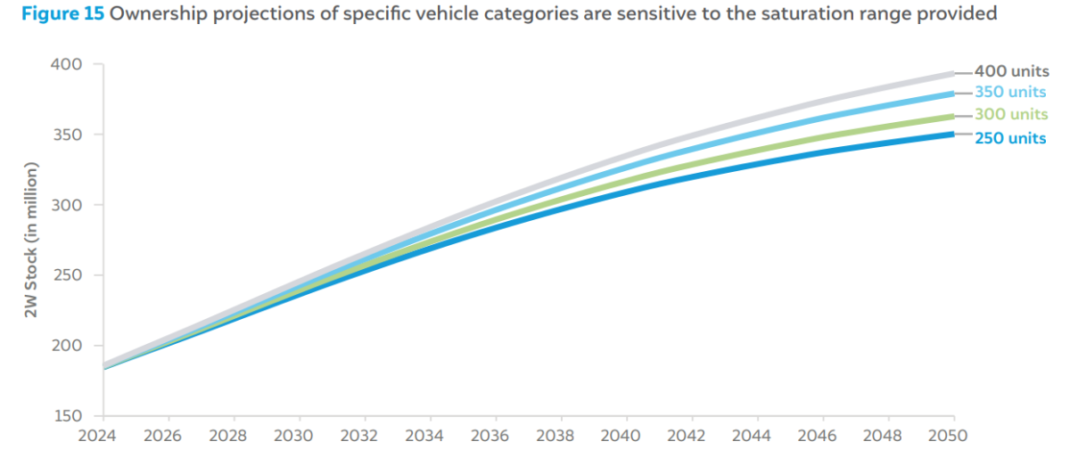
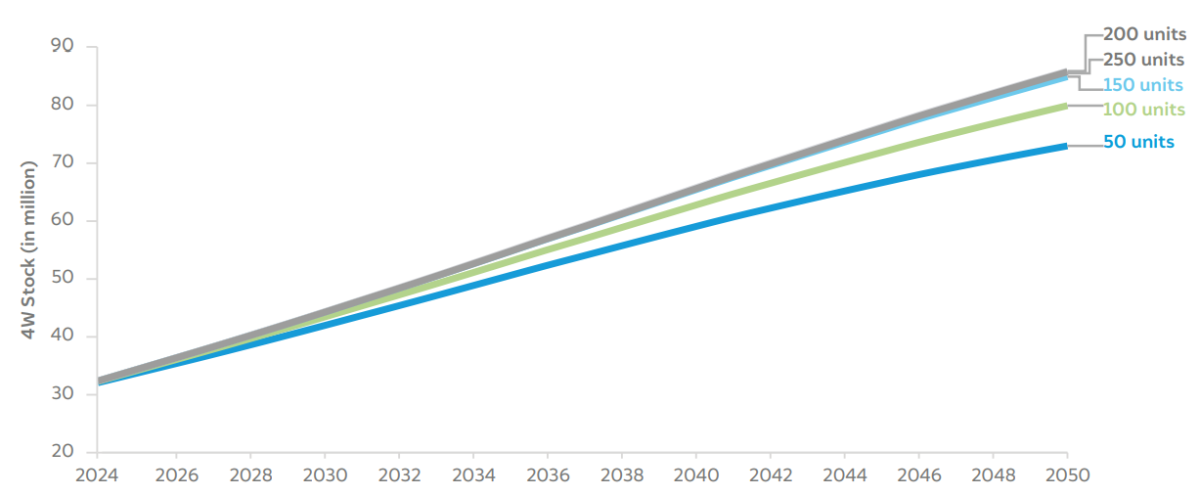
We conducted a sensitivity analysis to identify the effect of saturation limits on stock projections. The saturation limit was varied in increments of 25 or 50 to observe its effect on the stock. As we had mentioned earlier, the saturation and speed were provided as a range for the solver module in the sum of least squares approach to better fit the historical data. For the sensitivity analysis, the upper bound of the range was incremented by 25 or 50 units depending on the vehicle segment, and the results are illustrated in Figure 15.
In the 2W category, we expanded the upper limit of the saturation level in increments of 50 units, establishing four scenarios: 250 (baseline), 300, 350, and 400. Taking 250 per 1,000 people as our baseline scenario, we observed variations in the projected vehicle stock for 2050. Specifically, compared to the baseline, the 300-unit scenario resulted in a 4 per cent higher stock, the 350-unit scenario in an 8 per cent higher stock, and the 400-unit scenario in a 12 per cent higher stock in 2050.
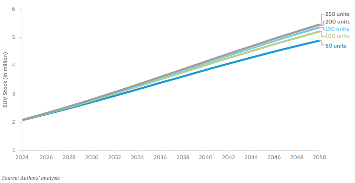
For the 4W segment, we increased/decreased the upper bound by 50, establishing five scenarios: 50, 100, 150 (baseline), 200, and 250. By 2050, stock increased by 1 per cent in the 200- and 250-unit scenarios, while it declined by 6 per cent and 14 per cent in the 100- and 50- unit scenarios, respectively. Similarly, for SUVs, the stock decreased by 9 per cent and 3 per cent in the 50- and 100-unit scenarios, while it increased by 1 per cent and 2 per cent in the 200- and 250-unit scenarios. Across other vehicle segments, the change in saturation range revealed minimal impact (between 1 and 2 per cent) on the overall stock as these segments had achieved optimal parameters.
The baseline was set at 250 per 1,000 people for 2W, and 150 per 1000 people for other vehicle categories, aligning with the saturation values used in the Soman, et al. (2020) study. The baseline values were selected from this study, as the shape parameters of the Gompertz equation were also derived from it.
We compared our vehicle stock estimates against the existing projections. Eight studies were chosen, including an estimate from a CEEW study conducted in 2020, as listed in Table 4.
Table 4 Studies used for comparison and validation of projections
| Published by | Study name (year) | Base year |
|---|---|---|
| CEEW 2020 | India’s electric vehicle transition—Can electric mobility support India’s sustainable economic recovery post-COVID-19? (2020) | 2016 |
| NITI-RMI | India Leaps Ahead: Transformative Mobility Solutions for All (2017) | 2015 |
| TERI | Roadmap for India’s energy transition in the transport sector (2024) | FY2019–20 |
| IIT | Projection of private vehicle stock in India up to 2050 (2019) | 2011 |
| CEEW-GCAM | Comparison and Decarbonisation Strategies for India’s Land Transport Sector: An Inter Modal Assessment (2019) | 2010 |
| PNNL | Comparison and Decarbonisation Strategies for India’s Land Transport Sector: An Inter Modal Assessment (2019) | 2010 |
| IRADe | Comparison and Decarbonisation Strategies for India’s Land Transport Sector: An Inter Modal Assessment (2019) | 2010 |
| IIMA-UNEP DTU | Promoting Low Carbon Transport in India (2014) | 2010 |
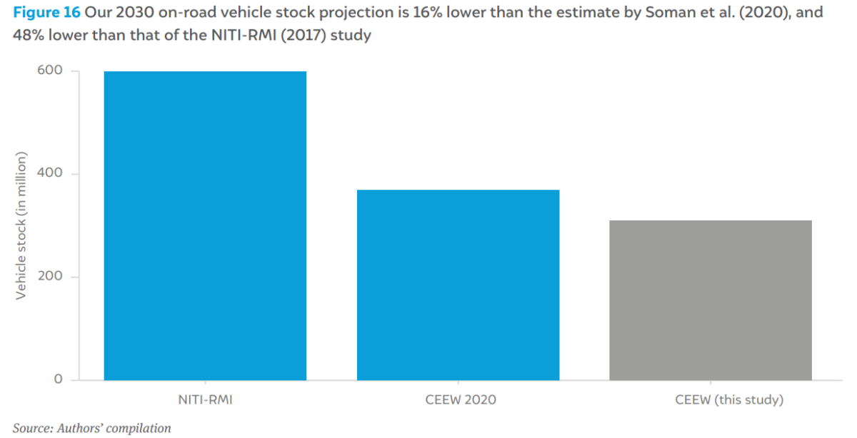
Our estimates are close to the previous forecast by CEEW (Soman et al. 2020). The differences can be attributed to using the same values of saturation and speed of adjustment in the mentioned study and the disruptive impact of COVID-19 on vehicular growth. Our estimates are 48 per cent lower than NITI-RMI’s (NITI Aayog and Rocky Mountain Institute) 2017 estimate. It is unclear whether the NITI-RMI study uses Gompertz to predict the future vehicle stock, but they have assumed a national GDP growth with a CAGR of 6.7 per cent to arrive at 598 million vehicles as of 2030.
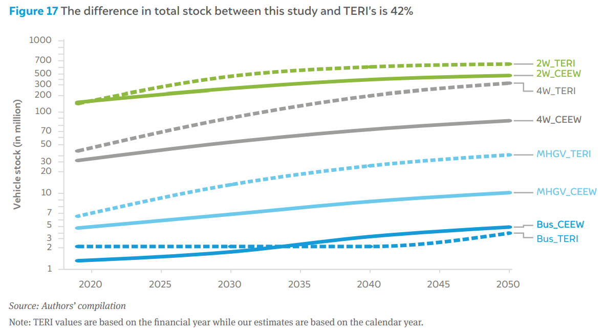
The comparison of overall stock estimates between this study and TERI for the year 2050 reveals a significant variation (The Energy and Resources Institute 2024). Our analysis projects the overall vehicle population to be 494 million in 2050 while TERI’s estimate is higher at 847 million, reflecting a variation of approximately 42 per cent. This variation can largely be attributed again to differences in methodology, particularly the use of singular saturation levels for the entire country in TERI’s study. The TERI study uses saturation levels of 300 per 1,000 people for 2W, 50 for 3W-P, 200 for 4W and SUV, and 25 for MHGVs. It applies these values at a national level. In contrast, our study derives the saturation level dynamically, based on historical patterns observed at district level. Additionally, a key distinction is that TERI uses a top-down approach to aggregate stock at the national level, whereas our study adopts a bottom-up approach to aggregate stock at the district level.
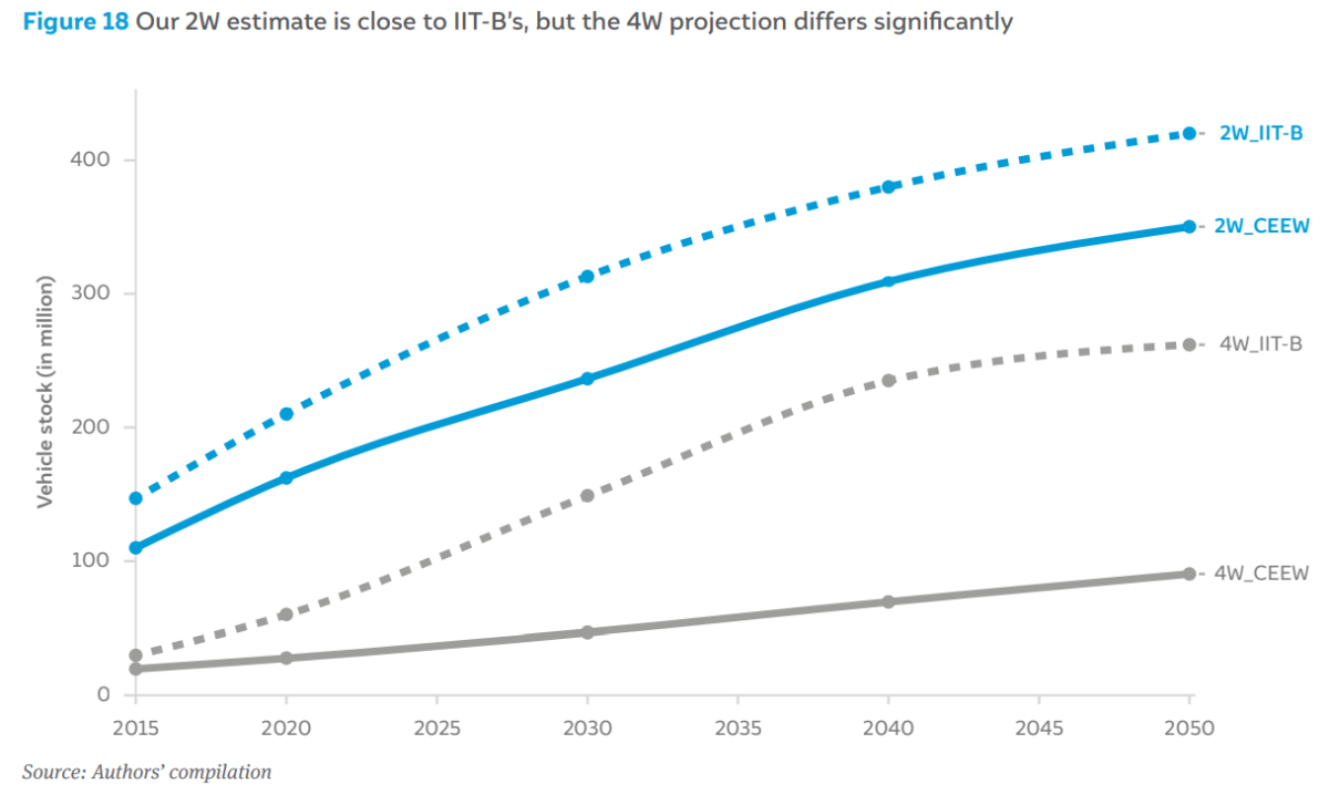
The 2W stock matches closer with the IIT-B estimates, with the variation largely constant in absolute terms through the future years (Singh, Mishra and Banerjee 2020). For example, the IIT-B study projected higher 2W stock by 34 per cent in 2015, and the difference narrowed to 32 per cent by 2030 and 20 per cent by 2050. The significant difference could be the base year and the difference in saturation values and speed of adjustment. The IIT-B study’s projection year starts in 2012, while in our study, the projection begins in 2024. Similarly, the IIT-B study uses a fixed saturation limit and speed of adjustment, while the two parameters in our study are chosen based on the best fit of the historical data.
In contrast, for the car segment (4W and SUV combined), the difference between our study and IIT-B estimates diverges from 2015. The IIT-B study projected car stock 51 per cent higher in 2015, rising to 218 per cent by 2030 and showing a marginal decline to 190 per cent by 2050. This is again due to the underlying assumptions in the model and the differences in the saturation and speed of adjustment values.
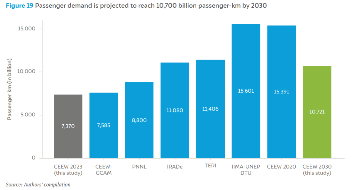
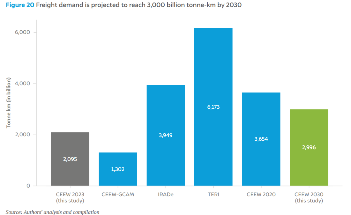
Beyond absolute vehicle stock, it is also important to examine other key metrics, such as total passenger demand and freight demand. The GDP per capita increase reflects not just on the number of vehicles, but also on the distance driven by the population. With growing affluence, leisure trips increase in distance and duration. Similarly, with increased industrialisation and consumption, the total tonnage of freight and distances goods are moved will increase. In 2023, the total passenger demand was approximately 7,370 billion kilometres, while the total freight demand was approximately 2,095 billion tonne-kilometres. By 2030, passenger demand is projected to rise to 10,700 billion kilometres, with freight demand reaching 3,000 billion tonne-kilometres.
Our passenger demand estimate match much closer with IRADe and TERI’s estimates. The difference between our estimates and those of the CEEW-GCAM model can be attributed to variations in modelling approaches, including their exclusion of taxis and other underlying methodological variations (CSTEP, CEEW, IRADe, PNNL, and TERI 2019).
As the Indian economy expands, the demand for mobility among the populace grows simultaneously. Consequently, transparent and reliable data on the vehicles plying on the road becomes an essential metric for policymakers to make informed decisions on infrastructure planning, environmental regulations, and transportation policies to manage the increased demand effectively.
Our analysis follows a bottom-up method of estimating vehicle stock at the district level. In our analysis, India’s growth pattern follows an S-shaped curve, with only the 2W category showing signs of saturation in the next 25 years. All other categories are at the lower end of the S-shaped curve and might reach saturation beyond 2050.
Without substantially more efforts to grow the share of public transport, the number of vehicles on the road will be high in 2050, and policy measures are imperative to control the negative externalities caused by them. As our analysis indicates, the country is in the initial stage of the Gompertz curve. Rising per capita income and the booming domestic automotive industry will only increase the vehicle population.
The major findings from this study include:
Historical stock calculations
Population projections
GDP projections
Gompertz function
Based on our methodology, limitations and findings from the stock projections, we recommend the following interventions.
Vehicle stock refers to the total number of registered vehicles that are actively on the road at a given point in time. It excludes scraped or decommissioned vehicles and represents the current fleet in use across different vehicle categories.
India had 226 million vehicles in 2023, including 175 million two-wheelers and 32 million private cars. Our analysis projects this to rise to 494 million by 2050, comprising 350 million two-wheelers and 90 million cars.
In 2023, Uttar Pradesh had the highest number of vehicles (29 million), followed by Maharashtra (21 million) and Tamil Nadu (19 million). By 2050, Uttar Pradesh is projected to reach 93 million vehicles—more than twice Maharashtra’s 43 million—while Bihar ranks third with 38 million.
How Secure is India’s Energy Future?
Unlocking the Potential for a Gas-Based Economy in India
Advancing India’s Green Steel Transition
CO₂ Pipeline Network for Carbon Capture and Storage in India

Bharat Cleantech Manufacturing Platform: Green Hydrogen Indigenisation Pathways