Council on Energy, Environment and Water Integrated | International | Independent
This study assesses Delhi’s air pollution scenario in the winter of 2021 and the actions to tackle it. Winter 2021 was unlike previous winters as the control measures mandated by the Commission of Air Quality Management (CAQM) in Delhi National Capital Region and adjoining areas were rolled out. These measures included the Graded Response Action Plan (GRAP) and additional emergency responses instituted on the basis of air quality and meteorological forecasts. Given that the forecasts play a major role in emergency response measures, the study assesses the reliability of different forecasts. Further, it gauges the impact of the emergency measures on Delhi’s air quality levels. It also discusses the primary driver of air pollution in winter 2021.
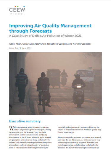
With every passing winter, the need to address Delhi’s air pollution grows more urgent. During the winter of 2021, the Supreme Court, the Delhi Government, and the Commission for Air Quality Management in the NCR and Adjoining Areas (CAQM), all sprang into action to arrest rising pollution levels in Delhi. The interventions ranged from shutting down power plants and restricting the entry of trucks into Delhi to school closures and using forecasts to pre-emptively roll out emergency measures. However, the impact of these interventions on Delhi’s air quality begs further investigation.
Through this study, we intend to examine what worked and what did not this season. As is the case every year, meteorological conditions played an important role in both aggravating and alleviating pollution levels. To assess the impact of meteorological conditions on pollution levels, we analysed pollution levels during the months of October to January vis-a-vis meteorological parameters. To understand the driving causes of pollution in the winter of 2021, we tracked the changes in relative contribution of various polluting sources as the season progressed.
While pre-emptive actions based on forecasts was a step in the right direction, an assessment of forecast performance is a prerequisite to integrating them in decision-making. We also assessed the performance of forecasts by comparing them with the measured onground concentrations. We also studied the timing and effectiveness of emergency directions issued in response to forecasts.
We sourced data on pollution levels from Central Pollution Control Board’s (CPCB) real-time air quality data portal and meteorological information from ECMWF Reanalysis v5 (ERA5). For information on modelled concentration and source contributions, we used data from publicly available air quality forecasts, including Delhi’s Air Quality Early Warning System (AQ-EWS) (3-day and 10-day), the Decision Support System for Air Quality Management in Delhi (DSS), and UrbanEmissions.Info (UE).
The number of ‘Severe’ plus ‘Very poor’ air quality days during the winter has not decreased in the last three years (Figure ES1). During the winter of 2021 (15 October 2021 - 15 January 2022), about 75 per cent of the days, air quality were in the ‘Very poor’ to ‘Severe’ category. Interestingly, despite more farm fire incidents in Punjab, Haryana, and Uttar Pradesh in 2021 compared to 2020, Delhi’s PM2.5 concentration during the stubble burning phase (i.e., 15 October to 15 November) was lesser in 2021. This was primarily due to better meteorological conditions like higher wind speed and more number of rainy days during this period.
We find that about 64 per cent of Delhi’s winter pollution load comes from outside Delhi’s boundaries (Figure ES2(a). Biomass burning of agricultural waste during the stubble burning phase and burning for heating and cooking needs during peak winter are estimated to be the major sources of air pollution from outside the city according to UE (Figure ES2(b). Locally, transport (12 per cent), dust (7 per cent), and domestic biomass burning (6 per cent) contribute the most to the PM2.5 pollution load of the city. While transport and dust are perennial sources of pollution in the city, the residential space heating component is a seasonal source. However, this seasonal contribution is so significant that as the use of biomass as a heat source in and around Delhi starts going up as winter progresses, the residential sector becomes the single-largest contributor by 15 December (Figure ES2(b)). This indicates the need to ramp up programmes to encourage households to shift to cleaner fuels for cooking and space heating.
Figure ES 2(a) Transport, dust, and domestic biomass burning are the largest local contributors to the PM2.5 pollution load in Delhi
Source: Authors’ analysis, source contribution data from DSS and UE.
Note: Modelled estimates of relative source contributions retrieved from UE and DSS.
Figure ES 2(b) Both local and regional sources need to be targeted for reducing Delhi’s pollution
Source: Authors’ analysis, source contribution data from UE.
Note: Source contribution data retrieved from UE district products which have larger geographical cover and lower resolution.
The availability of multiple forecasts provides decisionmakers with a range of options to choose from. At the same time, this is an obstacle to effective onground action. To streamline the flow of relevant information from forecasters to decision-makers, it is important to analyse the forecasts and assess their reliability. We found that all the forecasts identified pollution trends accurately (Figure ES3) but their accuracy in predicting pollution episodes (‘Severe’ and ‘Very Poor’ air quality days) decreases with future time horizon.
In November–December 2021, apart from the Graded Response Action Plan (GRAP) coming into effect in DelhiNCR, the CAQM introduced several emergency response measures through a series of directions and orders. The Supreme Court also stepped in from time to time to direct the authorities to act on air pollution.
As a first, the CAQM used air quality and meteorological forecasts to time and tailor emergency response actions. The first set of restrictions was put in place on 16 November 2021, and all were lifted by 20 December 2021, save the one on industrial operations.
Figure ES3 All the forecasts can predict the trend accurately
Source: Authors’ analysis, data from Central Pollution Control Board (CPCB), AQ-EWS, and UE.
Note: r represents correlation.
During this period, all the forecasts except AQ-EWS (3-day) underpredicted PM2.5 levels. Therefore, by looking at the difference between forecasted and measured concentrations, it is not possible to gauge the effectiveness of the restrictions conclusively. Hence, multiple models or different modelling experiments are needed to estimate the impact of the intervention.
It should be noted that during the restriction period, air quality did not descend into the ‘Severe +’ category. Further, when all the restrictions were in place along with better meteorology, air quality did improve from ‘Severe’ to ‘Poor’. The first prolonged ‘Severe’ air quality period in December was witnessed between 21 December and 26 December. While the forecasts sounded an alarm for high pollution levels during this period, all restrictions barring those on industrial activities were lifted. Subsequently, PM2.5 levels remained above 250 µgm-3 for six straight days resulting in the longest ‘Severe’ air quality spell of the season. (Figure ES4).
Figure ES4 The lifting of the restrictions was ill-timed with high pollution levels forecasted in the following days
Source: Authors’ analysis, data from Central Pollution Control Board (CPCB).
Note: C&D stands for construction and demolition activities. Work from home (WFH) stands for the 50% cap on employee attendance in the office. Industrial restrictions stand for compulsory switching over to Piped Natural Gas (PNG) or other cleaner fuels within industries and non-compliant industries being allowed to operate restrictively.
Over the past few years, Delhi’s winters have come to be synonymous with high pollution levels. This has attracted the attention of various stakeholders including policymakers, citizens, the media, multilateral agencies, and the judiciary. Delhi is among the few cities in India where both real-time and forecasted air quality data from multiple institutions are available. This, along with the acknowledgement of the problem at multiple levels of the government, underlines the relevance that air pollution has assumed in recent years. Despite this alignment of information and intent, 2021 was no different as the air quality remained ‘Poor’ to ‘Severe’ air quality categories for most of the winter. The worsening air quality prompted the CAQM to roll out a slew of restrictions that targeted, inter alia, construction activities, vehicular traffic, and power plants. These restrictions were based on air quality and meteorological forecasts. But given the high pollution load from local and regional sources, these emergency measures did not adequately arrest pollution episodes in the winter of 2021. This gives rise to multiple questions: why were emergency measures not able to prevent the worsening of air quality? What approach should be adopted to tailor the emergency response to pollution peaks?
Figure 1 How do cities around the world use air quality forecasts?

Air pollution is not unique to Delhi-NCR; many cities around the world, from Los Angeles to Paris to Beijing, grapple with this issue. Many of these cities use forecast-based alert systems to inform citizens and issue emergency measures in response to pollution episodes (Beijing Municipal Government 2020; Brussels Environment 2020; Madrid City Council 2018; Mexico City Government 2019; Mullins and Bharadwaj 2015). On the other hand, Delhi’s winter emergency response plan, Graded Response Action Plan (GRAP) is triggered by observed PM2.5 and PM10 concentrations. While a measurement-based system can only prevent further worsening of the situation, a forecast-based system can help avert pollution episodes and is, thus, more preferable.
At the national level, the National Clean Air Programme (NCAP), India’s flagship programme on air quality management, highlights the need for city-specific forecasting in all the non-attainment cities in the country. The forecasts can then be used to issue health alerts, supplement existing emission control programmes, and trigger emergency interventions to tackle high pollution episodes (Agarwal et al. 2020; Kurinji, Khan and Ganguly 2021; AQRS-CENR 2001). With the forecasts in place, the administration has the option to act pre-emptively and mitigate the risk posed by the episode by introducing curbs and measures.
For instance, the Indian Institute of Tropical Meteorology (IITM), Pune, developed the System of Air Quality and Weather Forecasting and Research (SAFAR) in collaboration with other Earth System Science Organisation (ESSO) institutions. SAFAR measures air quality in real-time and provides forecasts 1–3 days in advance for cities such as Delhi, Mumbai, Pune, and Ahmedabad (Beig et al. 2021; SAFAR 2021). More recently, the ESSO consortium, led by IITM and USA’s National Center for Atmospheric Research (NCAR), released an Air Quality Early Warning System (AQ-EWS) and a Decision Support System (DSS) to issue alerts and provide source contributions for Delhi (AQ-EWS 2021; DSS 2021; Jena et al. 2021). The Central Pollution Control Board (CPCB) also provides a 3-day forecast at the station level for Delhi. Then, there are also independent research groups like UE, founded by Dr Sarath Guttikunda, which provides city- and districtlevel forecasts along with source contributions for multiple cities, including Delhi (Guttikunda and Calori 2013; UE 2021).
Delhi is one of the few cities in India that have multiple forecasting systems. Ideally, the presence of multiple forecasts should drive the timing and tailoring of emergency responses to pollution episodes based on the predicted source contributions. Assessing the accuracy of these forecasts then becomes critical to utilise them to drive on-ground action. In 2021, apart from GRAP, a number of other restrictions were put in place based on forecasts. So, a comprehensive assessment of the accuracy of the forecasts as well as the emergency actions rolled out in the winter of 2021 is critical in understanding what worked and what did not.
To understand seasonal variations in source contribution estimates by these forecasts, we first assess the agreement between different forecasts and then compare them against ground observations. To do so, we use multiple datasets, including measured and modelled pollutant concentrations, meteorological data, and modelled source contributions from publicly available air quality forecasts for Delhi.
We obtained hourly PM2.5 concentrations from the Central Pollution Control Board (CPCB) real-time air quality data portal. Meteorological parameters like precipitation, temperature, wind speed, and boundary layer height (blh) were obtained from the European Centre for Medium-Range Weather Forecasts Reanalysis 5th Generation (ERA 5). Data on the number of fires was accessed from NASA’s Fire Information for Resource Management System (FIRMS) portal (NASA 2021). To assign air quality index (AQI) categories, only those monitoring stations that were operational across 2018–2021 and had ≥ 75 per cent data in a year were considered (Williams et al. 2014). As of January 2022, three forecasting services publicly provide air quality forecasts for Delhi NCT. These are AQ-EWS, SAFAR, and UE. A detailed description of the modelling inputs for each of the three systems is provided in Table 1.
Table 1 Different forecasts used in the study

To assess forecast performance, we compare modelled PM2.5 concentrations with the measured concentrations reported by the regulatory CAAQMS, Delhi. We use different statistical metrics to understand the goodnessof-fit of the forecast with the measured concentrations. The metrics include correlation coefficient (r), mean bias error (MBE), and the mean absolute percentage error (MAPE) (Koo et al. 2012; EPA 2007):
We also used accuracy as a metric to determine whether the forecast can predict the ‘Very poor’ and ‘Severe’ air quality categories. Accuracy here is defined as the number of correct predictions of the AQI category divided by the total number of predictions. We evaluate these metrics over different time horizons to examine how well the forecast performs for different time periods. Hence, we consider the first 24-hour forecast (day 1), the next 24-hour forecast (day 2), and the last 24-hour forecast (day 3) for the analysis. More information about the evaluation metric is given in the Annexure.
We also assess whether a model can capture spatial variations in pollution levels across the city. The spatial data file to us is available only for UE, we used that to assess station-level validation of the forecast. To do this, we first mapped the spatial grid of a forecast with the location of the regulatory monitor through a spatial intersection. Then, we calculated the performance metrics at each location with the intersecting grid. If more than one grid intersected, we calculated the average of the grids. Finally, we used the median of the metric across the stations to report the final performance.
We also attempt to evaluate if the pre-emptive emergency measures that were taken by CAQM and GNCTD had any impact on Delhi’s air quality. Additionally, we also explain the primary drivers that influence Delhi’s air quality this season — its sources and meteorological influences. For information on measures taken, we scanned through the directions and orders available on the CAQM website. We also perused relevant news articles that talked about the steps being taken to manage air pollution in the city.
2021 was marked by prolonged monsoons — the delayed retreat of the monsoons resulted in a longer clean air spell during the monsoon months and delayed the harvesting of crops in the north-western states of Punjab, Haryana, and Uttar Pradesh. With a drop in local wind speeds and an increase in the emission load from agricultural waste burning in nearby regions, Delhi’s air quality started deteriorating from the second week of October 2021. In response, CAQM ordered strict enforcement of the GRAP from 19 October 2021. Though the government increased vigilance, NCR’s air quality worsened further. The air quality breached the ‘Severe’ mark for five straight days following Diwali (4 November).
Finally, on 16 November 2021, CAQM came down heavily on polluting sources through its first emergency order of the season, which was followed by subsequent orders. Construction and demolition activities, freight and passenger traffic, and power plants and industries were the sectors targeted through this series of orders and directions. To facilitate compliance, CAQM also set up central and state-level task forces to enforce, monitor, and supervise the implementation of the orders and directions (CAQM 2021a; CAQM 2021b). In the following paragraphs, we discuss the air quality during this winter, the impact of meteorology, the contribution of different sources, and the performance of forecasts. Finally, we discuss upon whether the actions taken by CAQM resulted in any improvement in Delhi’s air quality.
Despite the aforementioned measures, Delhi’s air quality in the winter period (15 October 2021–15 January 2022) did not fare better than in the previous two years (Figure 2(a)). During the winter of 2021, about 75 per cent of the days, air quality was in the ‘Very poor’ to ‘Severe’ category. The city’s pollution hotspots, which were first identified in 2018, did not show any improvement compared to the last two years as well (Figure 2(b)). Please note that we have used nine hotspots in this analysis, selected using the criterion that ≥ 75 per cent of data is available in a year. This highlights the need for hyperlocal monitoring and clamping down of local sources. Even though stubble burning had a delayed start in 2021, around 85 per cent of the fires in Punjab, Haryana, and Uttar Pradesh happened during the stubble burning phase (i.e., 15 October – 15 November 2021). More details on the number of fires are given in the annexure.
We find that despite the region recording the highest number of fires in the last five years, Delhi’s air quality was better during the stubble burning phase in 2021 (i.e., 161 µgm-3) compared to 2020 (i.e., 214 µgm-3). This disproves the commonly held view that stubble burning is the primary contributor to the city’s winter pollution. Therefore, it is important to understand that improvement in air quality relies on how well yearround sources (both local and outside city boundaries) are managed. The contribution of sources during the winter is discussed in section 3.3.
Meteorological conditions play a crucial role in air quality, especially during winters. Low temperatures and ventilation parameters like wind speed and mixing layer height can prevent the dispersion of pollution. Given the impact winter meteorological conditions have on Delhi’s air quality, it would be premature to comment on changes in air quality without assessing the prevailing meteorological conditions. To explain how meteorology impacted pollution this season, we use a parameter called the ventilation index, which is a measure of the atmospheric potential to disperse pollutants. It is defined as the product of wind speed and mixing layer height. A higher ventilation index is favourable for dispersion while a low ventilation index results in the trapping of pollution. On comparing observed PM2.5 levels with hourly ventilation levels during the stubble burning phase, we see a negative correlation of about 0.4 between the PM2.5 concentration and ventilation Index (Figure 3).
Figure 2(a) No significant improvement in air quality days during winters in Delhi

Source: Authors’ analysis, data from Central Pollution Control Board (CPCB).
Figure 2(b) Delhi’s hotspots in 2021 did not fare any better compared to 2019 and 2020

The relatively lower concentrations during the stubble burning phase in 2021 despite a higher number of fires can also be explained by the relatively higher ventilation levels (Figure 3). Another meteorological factor that played a crucial role was rainfall. During 15–26 December 2021, the air quality was much worse than in 2020. However, the air quality improved substantially during 26 December 2021–15 January 2022, compared to the previous year, due to five rain and six trace rain days. More details on the impact of meteorology for respective phases are given in the annexure. While the impact of meteorological conditions on Delhi’s air quality can be demonstrated, these conditions cannot be controlled. Therefore, the only way to improve air quality is by cutting down emissions.
Figure 3 The stubble burning phase in 2021 had better air quality due to improved ventilation levels

Source: Authors’ analysis, pollutant data from Central Pollution Control Board (CPCB) and meteorological data from European Centre for Medium-Range Weather Forecasts (ECMWF).
To understand which sectors need to be targeted to cut down emissions and subsequently improve air quality, reliable information on emissions and source contributions is a must. For this study, we explore two such sources of information — IITM’s DSS and UE’s air quality forecasts for Delhi. In the following sections, we summarise and compare the information provided by both systems. Based on this comparison, we identify the key sources of pollution during the different phases of winter 2021.
Existing research on source contributions to Delhi’s pollution suggests that the relative contribution of different polluting sectors varies seasonally. Contributions also vary within the same season. To identify the key drivers of pollution in Delhi in 2021, we reviewed modelled source contribution estimates provided by IITM’s DSS and UE air quality forecasts for Delhi. We also used UE district level forecasts that has larger spatial coverage to study the sources outside the city boundary. Moreover, to understand the role of stubble burning, we also considered modelled estimates by SAFAR.
In 2021, there was significant debate around the actual contribution of stubble burning to Delhi’s pollution pie. The number of fires reported during the stubble burning phase in 2021 was the highest in the last five years. Cumulatively, about 80,000 farm fires were reported in Punjab, Haryana, and Uttar Pradesh during 15 October-15 November 2021.
We find that the average contribution of stubble burning during this period was around 17 per cent as per SAFAR, 32 per cent as per UE, and 12 per cent as per DSS. The estimates of the open fire relative contribution differ across the three models as each model considers different sector-wise absolute contributions that vary in terms of configuration (i.e., domain size and spatial resolution) and the emissions inventories they use. And, therefore, the relative contributions differ in value as well.
We find that about two-thirds of Delhi’s winter pollution comes from outside the city’s boundaries (Figure 4(a)). According to UE, biomass burning of agricultural waste during the stubble burning phase and burning for heating and cooking needs during the peak winter phase is estimated to be a major contributor to city’s pollution load(Figure 4(b)). Locally, transport (12 per cent), dust (7 per cent), and domestic biomass burning (6 per cent) contribute the maximum to the PM2.5 pollution load of the city. While transport and dust are perennial sources of pollution in the city, residential space heating is a seasonal source. But this seasonal contribution is so significant that, as the use of biomass as a heat source in and around Delhi starts going up as winter progresses, the residential sector becomes the single largest contributor in the peak winter phase (Figure 4(b)). It is important to note here that the DSS in the current form can apportion the share of nearby districts in Delhi’s pollution load. However, it does not identify the specific sources within these districts that need to be controlled. More details on the forecast contribution are given in the Annexures.
Figure 4(a) Transport, dust, and domestic biomass burning are the largest local sources of pollution in Delhi

Source: Authors’ analysis, source contribution data from DSS and UE.
Note: Modelled estimates of relative source contributions retrieved from UE and DSS.
Figure 4(b) Both local and regional sources need to be targeted for reducing Delhi’s pollution

Source: Authors’ analysis, source contribution data from UE.
Note: Data retrieved from UE district product which have larger coverage and lower spatial resolution.
The differences in the findings of the two forecasting models, UE and DSS, can be attributed to the different modelling inputs that the systems rely on. For instance, both systems use different emission inventories. The use of different inventories can result in significantly different modelled contributions of sources. As evidenced by previous assessments, existing emission inventories for Delhi vary significantly in their estimates for emissions from different polluting sectors (Jalan and Dholakia 2019).
Regardless of the variations in estimated source shares, it is clear that addressing transport-related emissions should be GNCTD’s priority. Firstly, restrictions on the movement of private vehicles should be introduced as soon as the models sound an alarm for ‘Very poor’ to ‘Severe’ air quality conditions in the coming days. Secondly, emissions related to space heating, both locally and in nearby districts, highlight how energy poverty in this region has unintended consequences for air pollution. Finally, emergency response measures should be enforced stringently across the NCR states. This will reduce the pollution load in the region and will benefit locally and across the Indo-Gangetic plain.
As mentioned previously, this was the first time forecasted air quality and meteorological conditions were considered while rolling out preventive measures. However, to integrate forecasts into decision-making, continuous validation of the forecast is critical. As described in the methodology section, we assess the performance of models by comparing the modelled and measured concentrations through different performance metrics.
From Figure 5, we can see that all the forecasts capture the trend in line with measured particulate concentration at the city level. In the case of the AQ-EWS (3-day) and AQ-EWS (10-day), the correlation is in the range of 0.54–0.87, while UE forecasts correlate in the range of 0.69–0.80. Moreover, all the forecast models have a mean absolute percentage error of less than 40 per cent. However, it is worth noting that all the models on average are underpredicting with respect to the average ground observations. Among all the forecasts, AQ-EWS (3-day) was found to have the lowest mean bias in the range of –3.7 µgm–3 to –9.5 µgm–3.
Accuracy in predicting high pollution episodes decreases for future time horizons
One of the main objectives of the forecast is to provide timely alerts specifically for high pollution episodes (‘Very poor’ and ‘Severe’ categories). We found that for day 1, the AQ-EWS (3-day) forecast can predict with an accuracy of 73 per cent while the AQ-EWS (10-day) forecast has an accuracy of 62 per cent (Table 2). In the case of UE, the accuracy is about 53 per cent. For day 2, the accuracy reduces for all the models – AQ-EWS (3-day) is about 56 per cent accurate, AQ-EWS (10-day) is 53 per cent accurate, while UE is about 44 per cent accurate. For day 3, for AQ-EWS (3-day), AQ-EWS (10- day), and UE, the accuracy reduced to 50 per cent, 42 per cent, and 36 per cent, respectively.
Figure 5 All forecasts can capture the trend but underpredict with respect to measured concentrations

Source: Authors’ analysis, data from Central Pollution Control Board (CPCB), AQ-EWS, and UE.
Table 2 The accuracy of forecasts decreases for future time horizons

Source: Authors’ analysis, forecast data from AQ-EWS and UE.
We find that AQ-EWS (3-day) has the lowest bias and the highest accuracy in predicting high pollution episodes. It is important to note that the AQ-EWS assimilates surface PM2.5 observations and MODIS AOD measurements to accurately determine the initial conditions, while the UE forecast system does not use any assimilation. While assimilation certainly improves model performance, the bias between predicted and measured concentrations helps diagnose the uncertainties in emission estimates that feed into the model.
Station-level validation of the forecast
PM2.5 concentration varies across the city due to multiple factors such as population distribution, land use, and local emission sources, i.e., the presence of small-scale industries, construction activities, traffic density, etc. To assess whether the modelled forecasts were able to capture this spatial variation in pollution levels, we compared modelled concentrations at monitoring station locations and the concentration reported by these monitoring stations. We consider the intersection of the spatial grids from UE’s and the location of regulatory monitors, and compare the modelled and measured concentrations. As seen in Figures 6 and 7, the model captures the trend reported by the regulatory monitors and performs reasonably across the regulatory locations. The forecast has a median correlation of about 0.69 and a median MAPE of 29 per cent. Further, the forecast does underpredict with a median bias of –25 µgm–3. Finally, the model can predict high pollution days with a median accuracy of about 54 per cent.
Figure 6 The model can capture the variation across the regulatory monitors

Source: Authors’ analysis, forecast data from UE.
Figure 7 The forecast performs reasonably across the regulatory monitors

Source: Authors’ analysis, forecast data from UE.
As discussed previously, emergency actions taken in 2021 ranged from a ban on construction sites, entry of diesel trucks into Delhi, temporary closure of power plants and industries, shutting down of schools, and mandating 50 per cent attendance in offices. The directions targeted a range of pollution sources. We find that all the forecasts except AQ-EWS (3-day) underpredict PM2.5 levels between 16 November 2021 and 20 December 2021, when all the restrictions were more or less in place simultaneously. With the existing information, it is not possible to gauge the effectiveness of the restrictions based on a comparison of forecasted and measured concentrations. Therefore, multiple models or different modelling experiments are needed to estimate the effectiveness of the intervention. However, it is interesting to note that while the restrictions were in place, air quality did not descend into the ‘Severe +’ category. Further, when all the restrictions were in place along with better meteorology, air quality did improve from ‘Severe’ to ‘Poor’. However, as soon as all the restrictions were lifted on 20 December 2021, the PM2.5 levels remained above 250 µgm–3 for the next six days (Figure 8). As seen in Figure 5, forecasts were able to sound an alarm for high pollution levels in the following days but the restrictions were lifted.
Figure 8 The lifting of the restrictions was ill-timed as high pollution levels were forecasted for the following days

Source: Authors’ analysis, data from Central Pollution Control Board (CPCB).
Note: C&D stands for construction and demolition activities. Work from home (WFH) stands for the 50% cap on employee attendance in the office. Industrial restrictions stand for compulsory switching over to Piped Natural Gas (PNG) or other cleaner fuels within industries and non-compliant industries being allowed to operate restrictively.
Using forecasts to drive ground-level action is not new in India — the IMD has used forecasts to roll out mitigation measures in the event of a cyclone since the institution’s establishment in 1875. Over the years, the cyclone warning system has undergone a sea change on the back of improvements in forecast accuracy as well as in standard operating procedure (SOP) driven mitigation measures. As a result, the loss of human life fell from around 10,000 (1999 Odisha cyclone) to around 20 (2013 cyclone Phailin) within 14 years (IMD 2019). With the Indian experience in forecast-based emergency responses to cyclones serving as a reference, we recommend the following to help the GNCTD and CAQM plan and execute emergency measures in response to pollution episodes:
The GRAP was launched in 2017 for Delhi NCR. It provides action protocols to be taken when the AQI reaches certain categories. However, it did not work effectively in Delhi because its actions are triggered by measured concentrations. On the other hand, in cities like Beijing and Brussels, emergency actions are announced based on forecasted concentrations. Therefore, GRAP must be redesigned such that actions are triggered by forecasted source contributions and forecasts of pollution peaks. It is evident that locally, transport and dust are the major contributors to Delhi’s pollution. Therefore, restrictions on the movement of vehicles should be introduced when air quality is forecasted to be in ‘Very poor’ and ‘Severe’ categories. Parking charges levied on private vehicles parked on public land in residential areas can be used to partially finance public transport subsidisation. For instance, in Brussels, public transport is made free for the entire period when ‘orange’ or ‘red’ alerts have been triggered (Brussels Environment 2021). Also, on forecasted ‘Very poor’ and ‘Severe’ air quality days, GNCTD can introduce the concept of ‘No Driving Day’ along the same lines as the ‘Hoy No Circula’ programme in Mexico City, where private vehicles are banned on one weekday per week depending on the last digit of the licence plate. This programme has been successful in reducing vehicular pollution in Mexico City (Molina et al. 2019). Similar best practices can be assessed and evaluated in Delhi and other non-attainment cities to tackle air pollution.
Domestic biomass burning was found to be one of the leading contributors of pollution in Delhi NCR, especially as winter progressed. Surveys can be done in residential areas across the NCR to assess the prevalence of the use of biomass for heating and cooking. Based on this, a targeted support mechanism must be evolved to allow households and others to use cleaner fuel for cooking and heating. Equally, there is a need to assess alternatives — specifically for space heating – and promote adoption among the larger public.
Individual-level action can be catalysed by relaying forecasts to the citizenry through social media platforms like Twitter, Facebook, and WhatsApp. The public can be encouraged to take preventive measures like avoiding unnecessary travel and wearing masks while stepping out. This will have the dual effect of reducing the individual’s exposure to pollution as well as on-ground activity levels.
The accuracy of the forecast in predicting pollution levels and source contributions depends largely on the emissions inventory used. However, there are uncertainties in emissions estimates and limitations in understanding local activities. Therefore, social media posts (texts and photos) and camera feeds from public places can be used to improve the accuracy of forecasts. For instance, the machine learning–based forecasting system developed by IBM and deployed in Beijing utilises social media posts and camera feeds to finetune its forecasts. The incorporation of pictures and text improved the accuracy of the forecasts by 20 per cent (Guerrini 2016). In India, and Delhi specifically, there are attempts to understand local sources where citizens can report polluting activities through the use of different apps like SAMEER, Green Delhi, and SDMC 311. Data from these apps can be incorporated into the model to improve the accuracy of the forecast. Ultimately, a crowd-sourced emissions inventory for the NCT of Delhi and the NCR will benefit modellers and policymakers alike while also making transparent the efforts to curtail polluting activity.
Weather prediction has improved substantially in the last few decades through the use of ensemble methods. An ensemble method is a probabilistic approach that takes the inputs from various forecasts and produces a measure of central tendency (Brasseur et al. 2019; Zhang et al. 2012). An important example is the ENSEMBLE system of the Copernicus Atmosphere Monitoring Service (CAMS), which is the regional forecasting service of the European Union’s earth observation programme, Copernicus. The ENSEMBLE system takes the forecasts of nine different chemical transport models (CHIMERE, EMEP, EURAD-IM, LOTOS-EUROS, MATCH, MOCAGE, SILAM, DEHM, and GEM-AQ) and produces the median of the forecast values at all grid points over Europe (Copernicus Atmosphere Monitoring Service 2020). CAQM can work collaboratively with air quality modellers and have an ensemble air quality forecast to drive action. This could improve the accuracy of air quality forecasts and lead to better coordination and engagement.
Though air pollution in Delhi is a year-round problem, the city experiences several pollution peaks during winter. 2021 was no different as air quality remained ‘Poor’ to ‘Severe’ for most of the winter. The worsening air quality prompted the CAQM to roll out a slew of restrictions that targeted construction activities, vehicular traffic, and power plants. Though these emergency response measures prevented the air quality from worsening to the ‘Severe +’ level, but still remained in ‘Very poor’ to ‘Severe’ categories during these restrictions.
Our analysis estimates how air quality in October 2021-January 2022 fared in comparison to the previous year. We find that the period from 15 November 2021 to 15 January 2022 mirrored the trend seen in the last few years. On the other hand, an improvement in the air quality in the stubble burning phase (i.e., from 15 October 2021 to 15 November 2021) was observed compared to last year. This improvement was largely driven by better atmospheric conditions compared to last year even though the number of fires in Punjab, Haryana, and Uttar Pradesh was higher than the last year. Since meteorology is beyond human control, the only way to improve air quality is by controlling emissions. We find that transport, dust, and domestic biomass burning are the largest local contributors to pollution in the city. The contribution from domestic biomass burning also increased as temperatures started dipping in late November. Understanding forecasted source contributions and pollution peaks are critical for targeted action. But having multiple forecasts, which is the case in Delhi, is an opportunity and barrier for effective on-ground delivery. Therefore, it is of paramount importance to assess the reliability of the available forecasts. We find in our analysis that all the forecasts can get the pollution trend right though underpredict pollution episodes (i.e., ‘Severe’ and ‘Very poor’ air quality days).
The year 2021 marked a first in the use of forecasts to guide decision-making in the capital’s air quality management sphere. The CAQM used meteorological and air quality forecasts to time and tailor emergency measures this winter. During restrictions, all forecasts except AQ-EWS (3-day) under predicted PM2.5. Hence, it is not possible to gauge the effectiveness of the restrictions based on the difference between forecasted and measured concentrations. Nevertheless, we highlight that lifting all the restrictions, except the one on industries, on 20 December 2021, was ill-timed with all the forecasts predicting high pollution levels in the following days. Aided by the worsening of meteorological conditions following 20 December 2021, the forecast turned out to be accurate as the PM2.5 levels remained above 250 µgm-3 for the next six days.
We emphasise the importance of calibrating response measures to forecasted source contributions and the need for timely roll-out of pre-emptive measures. This will eliminate the need for ad hoc ex-post measures under GRAP. We highlight that forecasts should be made available to citizens to encourage them to undertake localised efforts to improve air quality.
We recommend the incorporation of social media posts, camera feeds from public places, and data from various pollution-related grievance registration applications like SAMEER, Green Delhi, and SDMC 311 into forecasting models to improve their accuracy. The creation of a crowd-sourced emissions inventory for Delhi will be beneficial to both modellers and policymakers. We also recommend combining data from the multiple forecasts available for Delhi through the ensemble method, which outputs a summary statistic of the data that is input from multiple models. The ensemble approach could potentially yield better results than individual input models and can further allow CAQM to work in collaboration with forecasters.
Behaviour Change Approaches to Tackle Stubble Burning at Scale
Organic Waste Circular Economy for Viksit Bharat
How Can India Tackle Air Pollution with an Airshed-level Approach?
Roadmap of the methodology to assess the climate co-benefits of the SUP ban in Tamil Nadu
Roadmap of the methodology to assess the climate co-benefits of the SUP ban in Maharashtra