Council on Energy, Environment and Water Integrated | International | Independent
Suggested citation: Ignatious Sneha, Mohammad Rafiuddin. 2025. How Well Can Delhi Predict Air Quality? Insights for India’s Decision Support Systems: Council on Energy, Environment and Water.
In air quality management, the varied nature and voluminous data generated demand digital tools to simplify the analyses and provide actionable insights. Air Quality Decision Support Systems serve the purpose by integrating data from various sources and performing necessary analytics to support decision-making. In Delhi, the Commission for Air Quality Management in National Capital Region and Adjoining Areas (CAQM) relies on the Air Quality Early Warning System (AQEWS) and Decision Support System (DSS) for air quality decision-making during winter in Delhi.
This study analyses the AQEWS and DSS of Delhi, both qualitatively and quantitatively, to assess their performance during winter and summer between 2023 and 2025.
Air pollution is one of the greatest threats to public health. While short-term exposure can aggravate conditions such as asthma and impair lung function, long-term exposure can lead to chronic obstructive pulmonary disease (COPD), diabetes, and cancers, among other health issues (EEA 2024).
About 70 per cent of India’s population breathes air with the PM2.5 levels above the National Ambient Air Quality Standards (NAAQS) of 40 μg/m3 (S. Guttikunda and Ka 2022). To control air pollution in major cities, India launched the National Clean Air Programme (NCAP) in 2019, with a focus on 131 nonattainment cities (NACs) that do not meet the NAAQS. The increased attention to air pollution mitigation led to increased monitoring and, consequently, the generation of a large volume of air quality data. In India, air quality data is available from monitoring stations, source apportionment/emission inventory (SA/EI) studies, air quality forecasting models, satellite-based measurements, and other sources at various spatial and temporal scales.
Manual analysis of such voluminous data is impractical; hence, there is a need for digital tools to perform data analytics and provide actionable information. An air quality decision support system (AQDSS) serves this purpose. An AQDSS aggregates air quality data from different sources, performs the necessary analytics, and provides actionable insights to support air quality decision-making.
In the wake of Delhi’s worst smog episode in 17 years and a deadly dust storm in 2018, the Ministry of Earth Sciences (MoES) launched the Air Quality Early Warning System (AQEWS) in 2018 to provide air quality forecasts three days in advance for Delhi and select Indian cities. In 2021, the MoES launched a decision support system (DSS) for Delhi as an extension of the AQEWS. The DSS provides information on sectoral and regional contributions to Delhi’s PM2.5 levels during winter, including emissions from transportation, industry, and neighbouring districts. While the AQEWS provides forecasts of PM2.5 levels, the DSS complements it by providing information on the contribution of various sources. The Commission for Air Quality Management in National Capital Region and Adjoining Areas (CAQM) implements the Graded Response Action Plan (GRAP) in the Delhi NCR region based on the forecasts provided by the AQEWS and DSS.
Under the NCAP, the Ministry of Environment, Forest and Climate Change (MoEFCC) intends to commission AQEWS across all NACs. Apart from Delhi, seven other cities—Ahmedabad, Jaipur, Pune, Mumbai, Kolkata, Bengaluru, and Hyderabad—currently have similar operational AQEWSs. Given that Delhi’s AQEWS and DSS serve as models for other cities, assessing their effectiveness is essential. Therefore, through this study, we intend to analyse the performance of Delhi’s AQEWS and DSS in order to improve their effectiveness.
We assess the performance of Delhi’s AQEWS and DSS both qualitatively and quantitatively. We review the literature from around the world to identify the characteristics of an ideal AQDSS, and then we compare its features with those of Delhi’s AQEWS and DSS.
We also evaluate the AQEWS’s ability to accurately predict the air quality index (AQI) during winter 2023–24 and 2024–25. We compare the AQI forecast from the AQEWS with the observed AQI from the Central Pollution Control Board (CPCB). We then assess the ability of two forecasting models part of the AQEWS – namely, the Weather Research and Forecasting model coupled with Chemistry at 400-metre resolution (WRF-Chem (400 m)) and the India Meteorological Department’s System for Integrated Modelling of Atmospheric Composition (IMD SILAM) – to predict the hourly PM2.5 and PM10 accurately. To understand the system’s performance during different phases of winter, we analyse forecasts across four phases:
We also analyse the system’s performance during summer 2024.
Improving Delhi’s DSS would require incorporating actionable air pollution reduction scenarios, displaying the impact of GRAP restrictions, including sectoral contributions from NCR districts, and regularly updating emission inventories (EI). Additionally, a yearround operational DSS with open-access data and inclusion of specific chemical components of PM for advanced users will further aid independent research to improve Delhi’s AQEWS and DSS.
Figure ES1. The performance of the AQEWS in predicting the ‘severe and above’ category improved in 2024–25
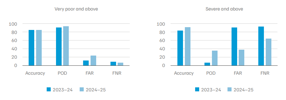
Source: Authors’ analysis
Note: POD = probability of detection. The ideal value for accuracy and POD for a model is 100%.
FAR = false alarm ratio. FAR is the rate at which a model falsely predicts pollution episodes. FNR = false negative rate.
FNR is the rate at which a model fails to predict pollution episodes. The ideal value for FAR and FNR for a model is 0%. The AQI data was not available for 13 days and 2 days from the AQEWS portal and CPCB, respectively, in 2024-25.
Air pollution is a significant global health burden, impacting 99 per cent of the global population (WHO 2024). It is the second leading risk factor for deaths worldwide, with a significant burden of disease in South Asia and Africa (HEI 2024). Global studies show that India is among the most polluted countries in the world, alongside many other developing countries (Gurjar 2021). According to the World Bank, the economic burden of illnesses linked to air pollution accounts for approximately 1.4 per cent of India’s gross domestic product (GDP) (World Bank 2024). Although air pollution levels in rural and urban environments can be similar (Basu 2023), the burden in cities is significantly higher due to their greater population density (Yuan et al. 2014). To address this, India launched the National Clean Air Programme (NCAP) in January 2019, aiming to reduce PM10 concentrations in cities by 20–30 per cent by 2024–25 (PIB 2024), relative to 2017 levels. This target was later revised to a 40 per cent reduction in PM10 levels by 2025–26 compared to 2019–20 levels (MoEFCC 2022).
India currently has 131 non-attainment cities (NACs) and million plus cities/urban agglomerations that do not meet the National Ambient Air Quality Standards (NAAQS), which indicate air quality levels considered safe for public health (PIB 2023).
The NCAP provided the impetus for cities to scale up air quality mitigation measures. According to the fourth National Apex Committee (September 2024), 95 out of the 131 cities showed at least a 1 per cent improvement in PM10 levels in 2023–24 compared to 2018–19 levels with 21 cities recording an improvement greater than 40 per cent (MoEFCC 2024). However, only 18 cities met the annual PM10 NAAQS value of 60 µg/m3. Successfully managing air quality requires cities to overcome administrative, governance, financial, and technical challenges, among others. Some of the key challenges are as follows:
The volume and varied nature of air quality data make manual analysis impossible. Therefore, cities require digital tools to analyse data and generate timely, actionable insights to support air quality decision-making. A decision support system (DSS) is one solution – a computer-based tool that supports decision-making through the automated analysis of data. While a DSS does not make decisions independently, it provides users with necessary information to inform their decision-making (Loucks 1995). Decision support tools improve transparency in the decision-making process and help quantitatively address the uncertainties involved (Sullivan 2002). Originally developed to support business decisions, the concept of DSS was extended to environmental systems due to the complex nature of environmental management. Thus, the term environmental decision support system (EDSS) emerged. An EDSS adopted in air quality management is an air quality decision support system (AQDSS).
India has been a pioneer in adopting state-of-the-art models and tools for air quality management. The System of Air Quality and Weather Forecasting and Research (SAFAR), under the Ministry of Earth Sciences (MoES), established an air quality forecasting system for Delhi during the 2010 Commonwealth Games (MoES 2009). The Indian Institute of Tropical Meteorology (IITM) and the India Meteorological Department (IMD) developed and operationalised an Air Quality Early Warning System (AQEWS) in 2018. The system provides three- to ten-day air quality forecasts for Delhi and six other cities – Mumbai, Pune, Ahmedabad, Kolkata, Hyderabad, and Bengaluru. In 2021, IITM and IMD developed a DSS for the Delhi NCR region.
Under the NCAP framework, all 131 NCAP cities aim to establish their own AQEWS (MoEFCC 2023). However, as of now, only eight cities in India have an operational AQEWS. This study analyses Delhi’s AQEWS and DSS to assess their potential for replication across other NCAP cities. Based on our analysis, we reflect on the characteristics of an effective AQDSS and provide recommendations for designing effective and sustainable systems for air quality management in Indian cities.
Despite the proliferation of DSSs in environmental management, their adoption remains limited (Zasada et al. 2017; Arnott et al. 2020). Walling and Vaneeckhaute (2020) categorised the key challenges associated with the success of an EDSS into three areas:
There are no universally defined factors attributed to the effectiveness of an EDSS. However, various studies examining the success and failure of different decision support tools have outlined some of the criteria associated with effective EDSSs. Since the system’s development aimed to support decision-making, the most critical factor for its success is its actual use by decision-makers. The number of users and their use of the system in decision-making for the intended purpose imply its success (Walling and Vaneeckhaute 2020). Wong-Parodi et al. 2020 reviewed the literature on DSS and synthesised the success criteria of an EDSS, as given in Table 1. We analyse what makes an AQDSS effective by drawing on this broader literature on EDSS success factors and challenges and Table 1 gives the criteria in detail.
Since an AQDSS is an EDSS, an ideal AQDSS should also possess the characteristics listed in Table 1.
Table 1. Characteristics of an effective environmental decision support system
| Characteristics | Description |
|---|---|
| The system must have a ‘clearly defined goal’. | • The system must have a well-defined objective (Wong-Parodi et al. 2020) and clearly identify the environmental problem it should address. |
| The system must ‘identify alternatives’. | • The system must identify and list the possible paths of action that are both technically and economically feasible (Sullivan 2002). |
| The system must ‘obtain relevant information’. | • The system must provide pertinent queries and results (Walling and Vaneeckhaute 2020). • The information supplied must be easily understandable to different stakeholders (Sullivan 2002), not just experts. |
| The system must ‘articulate values’. | • A DSS must convert data into meaningful and actionable information. The system must be able to produce understandable results and support the analyst in producing results that address end-user questions (McIntosh et al. 2011). |
| The system must ‘evaluate alternatives’. | • The system must not only identify the alternatives but also provide the impact of these choices based on the information obtained by the system (Wong-Parodi et al. 2020). |
| The system must ‘monitor the outcomes’. | • The system must review and monitor the outcomes and evaluate them (Wong-Parodi et al. 2020). • The outcome obtained on the ground also determines the success of a DSS developed to support decision-making in policy (McIntosh et al. 2011). |
Source: Authors’ compilation
Cities, states, and countries around the world use forecast-based AQDSSs to issue warnings and alerts or impose emergency measures to control emissions. Table 2 gives some global examples of AQDSSs.
Table 2. A review of air quality decision support systems around the world
Source: Authors’ compilation
Based on our review of AQDSSs across the world and the criteria that make an EDSS effective, we identify the components that an AQDSS should generally possess.
Air quality data
Air quality forecasts
Data analysis and visualisation
Recommendations
Scenarios
Response
Outcome monitoring
Air quality early warning and decision support system for Delhi
Delhi experienced its worst smog incident in 17 years in November 2016, with PM2.5 levels reaching 14 times the 24-hour NAAQS standard of 60 µg/m3 (EPCA 2017). In response, the Environment Pollution (Prevention and Control) Authority (EPCA) submitted a proposal to the Supreme Court (SC) for a smog alert system, drawing on international examples from China, the US, and France. The SC subsequently directed the CPCB and EPCA to develop an emergency response system for smog episodes. This led to the MoEFCC notifying the Graded Response Action Plan (GRAP) in January 2017. First implemented in the winter of 2017, GRAP outlined emergency interventions required under different AQI categories. Its purpose was to be a response plan to rising pollution rather than a substitute for long-term actions (EPCA 2017).
In 2018, the MoES launched an AQEWS for Delhi NCR to provide three-day air quality and weather forecasts (PIB 2018). Followed by this, in 2021, the ministry launched a DSS as an extension to the AQEWS to support decision-making for air quality management in Delhi and surrounding areas (IITM 2021). It provides source contributions to Delhi’s PM2.5 levels from 29 sectors, with a lead time of three days. The DSS complements the AQEWS: the AQEWS predicts pollutant concentrations, while the DSS attributes these concentrations to different sources. The CAQM, which replaced EPCA in 2020, formally linked GRAP implementation to the forecasts provided by the AQEWS and DSS in 2022 (Vibhaw 2022), marking a shift from reactive to proactive air quality management in Delhi. Currently, the information provided by the AQEWS and DSS guides the air quality management in the city during the winter season.
The AQEWS provides air quality forecasts and information on current air quality and weather conditions among others. Its major components are the following.
Air quality and weather data
Air quality and weather forecasts
Data analysis and visualisations
Figure 1. The Air Quality Early Warning System for Delhi portal displays information through line charts, maps, GIFs, etc.
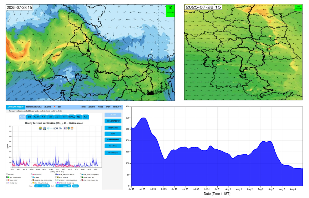
Indian Institute of Tropical Meteorology. Air Quality Early Warning System for Delhi. Ministry of Earth Sciences, Government of India. https://ews.tropmet.res.in/
The DSS linked to the AQEWS provides sectoral and regional contributions to Delhi’s PM 2.5 concentrations. Specifically, it estimates contributions from:
While the publicly available version of the DSS did not include an operational scenario module during the winter of 2024–25, it was operational in the previous year. In 2023–24, it offered users two scenarios to analyse the impact of source-level interventions on Delhi’s PM2.5 levels.
Figure 2. The scenario player on the Decision Support System (DSS) in the winter of 2023–24 showed potential improvement to Delhi’s PM2.5 with source-level interventions
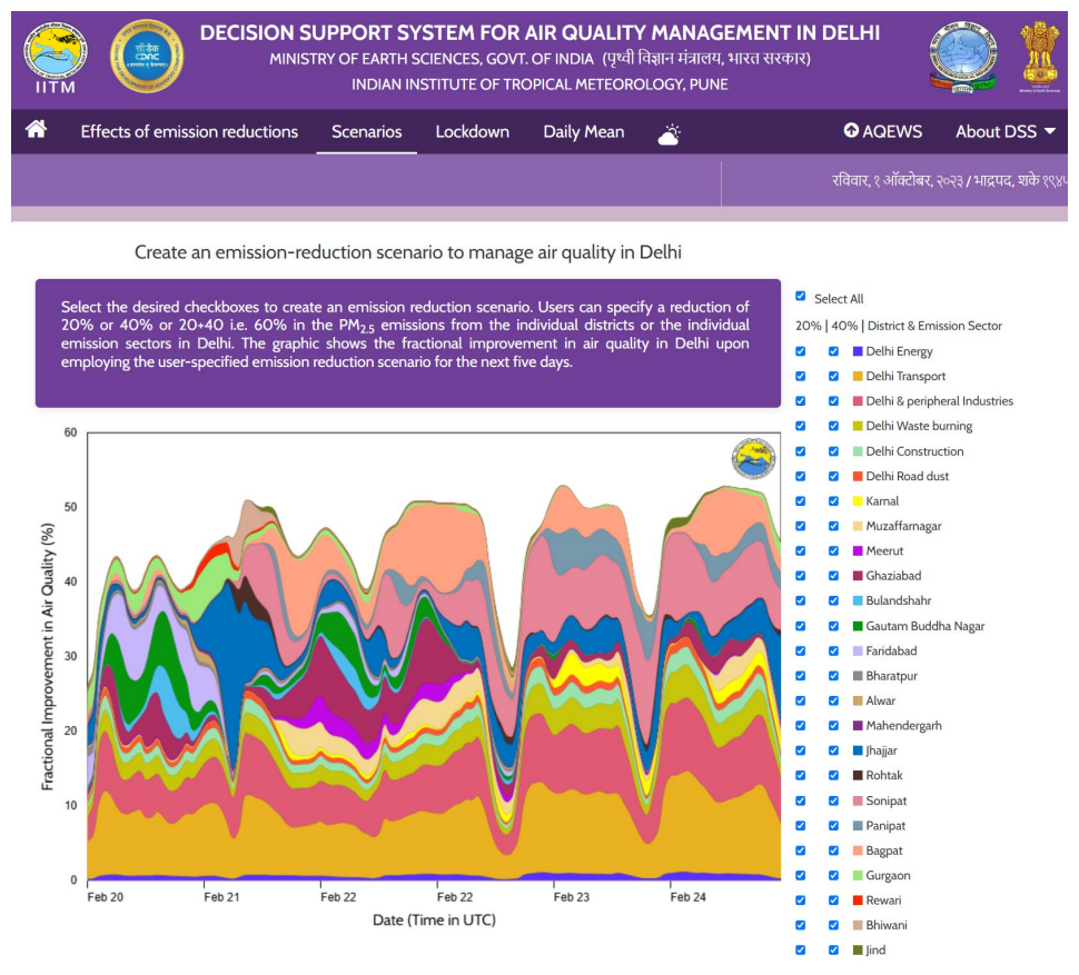
Indian Institute of Tropical Meteorology. Air Quality Early Warning System for Delhi. Ministry of Earth Sciences, Government of India. https://ews.tropmet.res.in/
As discussed earlier, the CAQM considers the data from the AQEWS and DSS before imposing the GRAP. The GRAP schedule consists of four stages, with increasing severity of restrictions based on air pollution levels. Figure 3 shows the AQI categories and the corresponding stages of GRAP.
Figure 3. AQI categories and corresponding GRAP stages
Source: Commission for Air Quality Management in National Capital Region and Adjoining Areas. Graded Response Action Plan (GRAP) for the National Capital Region (NCR). New Delhi: CAQM, 2024.
Under Stage I, the GRAP requires construction sites to strengthen the implementation of dust mitigation measures. It mandates the authorities to regularly clear solid waste and construction and demolition waste, along with periodic mechanised sweeping and water sprinkling on roads.
Stage II calls for the intensified implementation of Stage I measures and targeted action across air pollution hotspots in the Delhi NCR region. Additional measures are introduced at this stage to promote and augment public transport.
Stage III prohibits construction activities and imposes restrictions on entry of vehicles using unclean fuels into Delhi.
Stage IV prohibits the entry of polluting vehicles into Delhi and allows government employees to work from home.
We evaluate Delhi’s AQEWS and DSS using both qualitative and quantitative parameters. For the qualitative assessment, we compare the features of the AQEWS and DSS with those of an ideal AQDSS listed in Table 1. For the quantitative evaluation, we compare the ability of the forecasts from AQEWS to accurately predict both the AQI category and pollutant concentrations. To this end, we scrape the ‘Day 1’ forecast data from the AQEWS web portal for the 2023–24 and 2024–25 periods.
The forecasted AQI on AQEWS is from the WRF-Chem model, which operates at a spatial resolution of 400 metres (WRF-Chem 400 m). The AQI displayed corresponds to the higher of the two AQI values computed from forecasted PM2.5 and PM10 concentrations. To assess the model’s ability to forecast AQI categories accurately, we rely on the metrics listed in Table 3. Annexure 1 provides the confusion matrix and the formulae used to compute these metrics. We restrict our evaluation to two categories – ‘very poor and above’ (AQI > 300) and ‘severe and above’ (AQI > 400). ‘Severe and above’ is a subset of ‘very poor and above’. GRAP contains stringent measures under Stages II, III and IV, and the CAQM imposes these stages when the AQI crosses 300. Therefore, we restrict the evaluation to the above two categories. Moreover, according to the CPCB, an AQI above 300 has an adverse impact on the general population (Annexure 2). Since CPCB’s AQI is the average AQI between 4 PM of a given day and 4 PM of the previous day, we similarly compute the average forecast AQI for comparison.
Table 3. Metrics used to assess the ability of the forecasts to predict the AQI
Source: Authors’ compilation
To assess the ability of the AQEWS to accurately forecast pollutant concentrations, we compare the PM2.5 and PM10 forecasts from the WRF-Chem (400 m) and IMD-SILAM models with the actual concentrations observed in Delhi. To analyse the performance, we compute the metrics listed in Table 4. We obtain the actual PM2.5 and PM10 values from the AQEWS through web scraping. Both models provide spatially averaged hourly forecasts for PM2.5 and PM10 concentrations over Delhi. Although the AQEWS hosts 13 models for PM2.5 and 8 models for PM10 on its web portal, we limit our discussion to WRF-Chem (400 m) and IMD-SILAM. This is because the IMD issues air quality and weather forecast bulletins based on the IMD-SILAM model output, and the DSS runs on the WRF-Chem (400 m) model. Moreover, most other models on AQEWS do not offer continuously available data.
We analyse forecast performance for winter 2023–24 and 2024–25 (October–February). Also, we analyse the performance for summer 2024–25 (May and June). Additionally, to assess if the forecast performance varies during different periods within winter, we break the winter period into four phases. These phases are ‘stubble burning phase’ (16 October–30 November), ‘post-stubble burning phase’ (1 December–15 December), ‘peak winter phase (16 December–15 January) and ‘post-peak winter phase’ (16 January–28 February).
Table 4. List of metrics used to analyse the performance of the AQEWS to predict the pollutant concentration
Source: Authors’ compilation
In June 2024, the Rajasthan State Pollution Control Board (RSPCB) launched an AQEWS and DSS covering Jaipur city and its surrounding districts (The Times of India 2024). Similarly, Gujarat plans to extend an AQEWS to all industrial towns and NACs (Dave and John 2025).
India is also part of the World Meteorological Organization’s Global Atmosphere Watch (GAW) Programme, specifically the Global Air Quality Forecasting and Information System (GAFIS), which aims to provide air quality forecasting information in a globally harmonised and standardised way tailored to society’s need (WMO, n.d.). Delhi’s system thus serves as a model for countries that are yet to adopt forecasting systems. This highlights the need to evaluate the performance of Delhi’s operational AQEWS and DSS, both qualitatively and quantitatively. While IITM/IMD has conducted a quantitative evaluation of the system, it was limited to the postmonsoon winter months between October and January, using data from 2019 to 2024.
Table 5 presents a comparison of the features of Delhi’s AQEWS and DSS with those of an ideal AQDSS.
Table 5. Delhi’s Air Quality Early Warning System and decision support system satisfy most requirements of an ideal air quality decision support system
Source: Authors’ analysis
We observe that the AQEWS and DSS align well with most characteristics of an ideal AQDSS. They have a clearly defined goal – to support air pollution mitigation through forecasts. The systems integrate and analyse large volumes of air quality and weather information and disseminate it to the public in accessible formats. In 2023–24, the DSS enabled users to examine the impact of source-level reductions. However, it did not outline actionable pathways to achieve those reductions. Similarly, while AQEWS incorporated GRAP interventions into its forecasts, the system does not monitor the outcomes.
AQI prediction performance during winter
Winter 2023–24 recorded 92 days classified as ‘very poor and above’, including 15 ‘severe and above’ days. Annexure 3 presents the number of days in each category, along with the corresponding AQI predictions. The WRF-Chem (400 m) forecasts accurately predicted the AQI under both categories more than 80 per cent of the time in winter 2023– 2024. Its POD exceeded 90 per cent for the ‘very poor and above’ category but dropped to around 7 per cent for ‘severe and above’. Moreover, the FAR for ‘severe and above’ was greater than 90 per cent. Table 6 summarises the model’s performance in forecasting AQI categories during winter 2023–24.
Table 6. Performance of Delhi’s Air Quality Early Warning System in winter 2023–2024
Source: Authors’ analysis
According to the IITM/IMD analysis of the system’s performance during the post-monsoon months between 2019 and 2024, the accuracy of the system in predicting ‘very poor and above’ and ‘severe and above’ categories was approximately 80 per cent. The FAR for ‘very poor and above’ was around 18 per cent, while that for ‘severe and above’ was about 42 per cent. The POD of ‘very poor and above’ was 94 per cent, and 33 per cent for ‘severe and above’ (Ghude et al. 2024).
Our analysis shows that in winter 2024–25, the AQEWS’s ability to forecast ‘severe and above’ episodes improved. The accuracy under this category rose to 91 per cent from 83 per cent in 2023–24. The FAR dropped to 37 per cent from 91 per cent, and the POD increased to 36 per cent from around 7 per cent. The FNR also improved to 0.64 from 0.93. While the system correctly predicted only 1 out of 15 ‘severe and above’ days in 2023–24, it accurately predicted 5 out of 14 such episodes in 2024–25.
However, the metrics for ‘very poor and above’ remained the same in 2024–25 compared to 2023–24. Accuracy remained same at about 85 per cent, the FAR increased to 24 per cent, and the POD increased to 93 per cent. Similarly, the FNR marginally improved to 0.07. This suggests that while the system’s performance in predicting air pollution episodes with AQI between above 300 remained the same, its ability to forecast AQI levels above 400 improved substantially. Table 7 summarises the WRFChem (400 m) model’s performance in forecasting AQI during winter 2024–25. Figure 4 presents a comparison of the system’s performance across the 2023–24 and 2024–25 periods.
Table 7. Performance of Delhi’s Air Quality Early Warning System in winter 2024–25
Source: Authors’ analysis
Note: The AQI data was not available for 13 days and 2 days from the AQEWS portal and CPCB, respectively, in 2024-25.
We conclude that when the AQEWS forecasts the AQI to be ‘very poor and above’, the observed AQI is likely to fall within the ‘very poor’, ‘severe’, or ‘severe plus’ categories with high probability.
Figure 4. The accuracy of predicting the ‘severe and above’ category improved in 2024–25 but remained the same for ‘very poor and above’
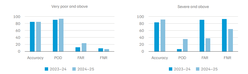
Source: Authors’ analysis
Note: POD = probability of detection; FAR = false alarm ratio; FNR = false negative rate. The AQI data was not available for 13 days and 2 days from the AQEWS portal and CPCB, respectively, in 2024-25.
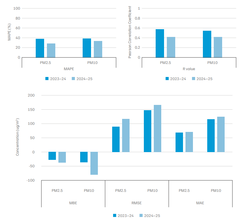
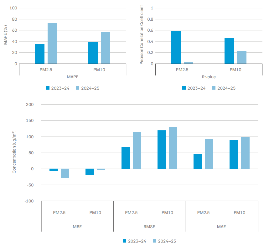
According to the IITM/IMD analysis of the model’s performance in predicting PM2.5 during the postmonsoon months between 2019 and 2024, the RMSE for PM2.5 was approximately 70 µg/m3 (Ghude et al. 2024). While Ghude et al. (2024) computed additional metrics such as the index of agreement (IOA), mean fractional bias (MFB), normalised mean bias (NMB), normalised mean square error (NMSE), we calculate the MAPE, MAE, MBE, and R value.
In 2023–24, the MAPE of PM 2.5 and PM10 forecasts from the WRF-Chem model (400 m) was 35 per cent and 37 per cent, respectively. For the IMD SILAM Figure 4. The accuracy of predicting the ‘severe and above’ category improved in 2024–25 but remained the same for ‘very poor and above’ model, the MAPE was around 49 per cent for PM2.5 and 38 per cent for PM10. The MBE of PM2.5 and PM10 forecasts from WRF-Chem (400 m) were around −18 µg/m3 and −34 µg/m3 , respectively. For the IMD SILAM model, the MBE was 0.67 µg/m3 for PM2.5 and −29 µg/m3 for PM10. Tables 8 and 9 present the metrics for the WRF-Chem (400 m) and IMD SILAM models, respectively, for the period 2023–24. While the two models displayed comparable performance for PM 10, their performance for PM2.5 differed significantly. Other metrics listed in Table 8 reflect the same. Notably, the Pearson correlation (R value) between the forecasts and observations was stronger for the WRF-Chem (400 m) model (0.59 and 0.54 for PM2.5 and PM10, respectively) compared to the IMD SILAM model (0.37 and 0.42 for PM2.5 and PM10, respectively).
Table 8. Performance of WRF-Chem (400 m) during winter 2023–24
Source: Authors’ analysis
The total number of hourly readings for PM2.5 and PM10 during this period2 was 3,120. The average observed PM2.5 concentration, corresponding to available WRF-Chem (400 m) data, was 181 µg/m3 , while the average predicted PM2.5 concentration from the model was 163 µg/m3 . For PM10, the average observed PM10 concentration was 304 µg/m3 , and the corresponding average predicted PM10 concentration was 270 µg/m3.
The total number of hourly readings for PM2.5 and PM10 during this period was 2,916. The average observed PM2.5 concentration, corresponding to available IMD SILAM data, was 179 µg/m3, while the average predicted PM2.5 concentration from IMD SILAM was 180 µg/m3. For PM10, the average observed PM10 concentration was 303 µg/m3, corresponding to available IMD SILAM data, and the average predicted concentration from IMD SILAM was 273 µg/m3.
In winter 2024–25, the performance of the WRFChem (400 m) model in predicting PM2.5 and PM10 remained largely unchanged. The MBE for PM2.5 deteriorated by 7 µg/m3, and by 25 µg/m3 in the case of PM10. The RMSE value for PM2.5 worsened to 93 µg/m3, whereas it worsened to 136 µg/m3 in the case of PM10. While the correlation between PM2.5 forecasts and actual values remained unchanged, the correlation between PM10 forecasts and actual values improved from 0.54 to 0.6. Conversely, PM2.5 forecasts from the IMD SILAM model improved on all metrics in 2024–25 except for MBE, while PM10 forecasts deteriorated on all metrics except for R values (correlation).
We therefore conclude that the WRF-Chem (400 m) model outperforms the IMD SILAM model in forecasting both PM2.5 and PM10. However, the negative MBE values from WRF-Chem (400 m) indicate consistent underprediction during both winters. Tables 10 and 11 summarise the performance of both models in 2024–25. Seven other Indian cities now have an operational AQEWS, and we present the analysis for these cities in Annexure 4.
Table 10. Performance of WRF-Chem (400 m) during winter 2024–25
Source: Authors’ analysis
The total number of readings for PM2.5 and PM10 during this period3 was 2,598 (hourly data). The average observed PM2.5 concentration was about 175 µg/m3, and the average predicted PM2.5 concentration from WRF-Chem (400 m) was 149 µg/m3. In the case of PM10, the average observed PM10 concentration was 292 µg/m3 , and the average predicted PM10 concentration from WRF-Chem (400 m) was 231 µg/m3.
Table 11. Performance of IMD SILAM during winter 2024–25
Source: Authors’ analysis
The total number of hourly readings for PM2.5 and PM10 during this period was 2,173 and 2,170, respectively. The average observed PM2.5 concentration was 177 µg/m3, corresponding to available IMD SILAM data, while the average predicted PM2.5 concentration from IMD SILAM was 154 µg/m3. For PM10, the average observed concentration was 306 µg/m3, and the average predicted PM10 concentration from IMD SILAM was 363 µg/m3.
A recent study led by IITM notes that uncertainties associated with emissions from large-scale stubble burning during the post-monsoon months contribute to a deterioration in forecast accuracy. Moreover, these uncertainties compound those arising from the simulation of weather variables, such as wind speed, temperature, and planetary boundary layer height (PBLH). The study found that the system performs exceptionally well on the first and second days, and moderately well on the third day (Ghude et al. 2024).
We assessed the AQEWS’s performance across four phases of winter – ‘stubble burning phase’, ‘poststubble burning phase’, ‘peak winter phase’, ‘postpeak winter phase’. Tables 12 and 13 present the phase-wise analysis results for PM2.5 and PM10, respectively.
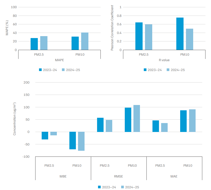
In 2023–24, the MAPE for predicting PM2.5 and PM10 was around 37 per cent during the stubble burning phase. It improved to 28 per cent for PM2.5 and 33 per cent for PM10 in 2024–25. However, despite this improvement in MAPE, all other metrics during this phase deteriorated in 2024–25 compared to 2023–24. The MBE for PM2.5 declined to −36 µg/m3 in 2024–25 from −26 µg/m3 in 2023–24. Similarly, for PM10, the MBE worsened to −80 µg/m3 in 2024–25 from −35 µg/m3 in 2023–24. The RMSE values for PM2.5 and PM10 also worsened by 27 µg/m3 and 18 µg/m3, respectively, in 2024–25. The MAE for PM2.5 and PM10 deteriorated by 2 µg/m3 and 9 µg/m3, respectively, in 2024–25. Additionally, the R value for both PM2.5 and PM10 worsened from 0.5 in 2023–24 to 0.42 in 2024–25.
Figure 5. The mean absolute percentage error during the stubble burning phase improved for both PM2.5 and PM10 in 2024–25, whereas the other metrics deteriorated
Source: Authors’ analysis
In 2023–24, the MAPE during the post-stubble burning phase for PM2.5 and PM10 were 27 per cent and 31 per cent, respectively. However, in 2024–25, it deteriorated to 32 and 41 per cent for PM2.5 and PM10, respectively. The performance of MBE, RMSE and MAE during this phase improved for PM2.5 in 2024–25 but deteriorated for PM10. The MBE for PM2.5 improved to −14 µg/m3 from −30 µg/m3 , and the RMSE value improved to 48 µg/m3 from 57 µg/m3 . Similarly, the MAE for PM2.5 improved to 36 µg/m3 in 2024–25 from 47 µg/m3 of the previous year. The RMSE value of PM10 worsened by 10 µg/m3 in 2024–25, whereas the MBE and MAE worsened by around 5 µg/m3 . While the R value of PM2.5 remained largely unchanged in 2024–25, it worsened to 0.49 from 0.75 in the case of PM10.
Figure 6. The performance of the WRF-Chem (400 m) model to predict PM10 deteriorated in 2024–25
Source: Authors’ analysis
Table 12. Phase-wise performance of air quality early warning system in predicting PM2.5 in 2023–24 and 2024–25
Source: Authors’ analysis
Note: Orange and green colours indicate deterioration and improvement in 2024–25 compared to 2023–24, respectively.
Table 13. Phase-wise performance of air quality early warning system in predicting PM10 in 2023–24 and 2024–25
Source: Authors’ analysis
Note: Orange and green colours indicate deterioration and improvement in 2024–25 compared to 2023–24, respectively.
The MAPE for PM2.5 and PM10 during the peak winter phase in 2023–24 was 33 per cent. In 2024–25, it deteriorated to 35 per cent and 38 per cent for PM2.5 and PM10, respectively. The MBE for both PM2.5 and PM10 during this phase remained unchanged during both winters. It was around −20 µg/m3 for PM2.5 and −40 µg/m3 for PM10. The RMSE and MAE values improved for both PM2.5 and PM10 in 2024–25 compared to 2023–24. The RMSE values for PM2.5 improved to 73 µg/m3 in 2024–25 from 90 µg/m3 in 2023–24. In the case of PM10, it improved to 120 µg/m3 in 2024–25 from 147 µg/m3 in 2023–24. Similarly, the MAE for PM2.5 and PM10 improved by 12 µg/m3 and 23 µg/m3 , respectively, in 2024–25. Moreover, the R value of PM2.5 improved to 0.75 in 2024–25 from 0.42 in 2023–24. Similarly, it improved to 0.69 in 2024–25 from 0.43 in 2023–24.
Figure 7. The Pearson correlation coefficient (R value) for both PM2.5 and PM10 improved in 2024–25
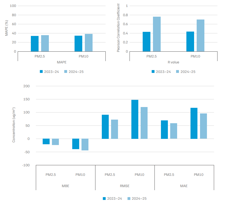
Source: Authors’ analysis
The MAPE for PM2.5 and PM10 during the postpeak winter phase was 36 per cent and 39 per cent, respectively. It deteriorated to 73 per cent and 57 per cent for PM2.5 and PM10, respectively, in 2024–25. The MBE for PM2.5 and PM10 in 2023–24 was −6 µg/m3 and −18 µg/m3 respectively. While the MBE for PM2.5 deteriorated to −27 µg/m3 in 2024–25, it improved to −4 µg/m3 for PM10. The RMSE values for PM2.5 and PM10 in 2023–24 were 67 µg/m3 and 119 µg/m3 , respectively. However, it worsened by 46 µg/m3 for PM2.5 and by 11 µg/m3 for PM10 in 2024–25. Similarly, the MAE values also deteriorated for both PM2.5 and PM10. For PM2.5, it worsened by two times to 91 µg/m3 in 2024–25 from 47 µg/m3 in 2023–24. Similarly, it worsened to 100 µg/m3 from 88 µg/m3 in the case of PM10. Similarly, the R value of PM2.5 worsened to 0.03 in 2024–25 from 0.58 in 2023–24, whereas it worsened to 0.22 from 0.46 in the case of PM10.
Figure 8. The performance of the air quality early warning system in predicting both PM2.5 and PM10 during post-peak winter phase deteriorated in 2024–25 compared to 2023–24
Source: Authors’ analysis
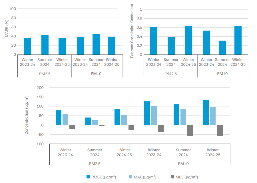
We analysed the performance of the AQEWS in forecasting pollutant concentration in summer (May– June). Table 14 summarises the results of our analysis.
The PM2.5 and PM10 observations during this period were available for 1,400 hours.5 The average observed PM2.5 concentration was 76 µg/m3, corresponding to available WRF-Chem (400 m) data, while the average predicted concentration was 72 µg/m3. In the case of PM10, the average observed concentration was 222 µg/m3, and the average predicted concentration was 167 µg/m3 .
Table 14. The WRF-Chem (400 m) model recorded a mean absolute percentage error of about 40% in summer 2024
Source: Authors’ analysis
The MAPE for PM2.5 during summer 2024 was 42 per cent, about a 6 per cent increase from that of winter 2023–24 and 2024–25. Similarly, the MAPE for PM10 during summer was 45 per cent, about 7 per cent higher than winter 2023–24 and 2024–25. Moreover, the R value worsened to 0.39 and 0.3 for PM2.5 and PM10 during summer 2024, whereas it was above 0.5 for both during winter 2023–24 and 2024–25. Despite the decline in MAPE and R values in summer 2024, the RMSE and MAE values for PM2.5 and PM10 improved in summer 2024 compared to winter 2023–24 and 2024–25. The RMSE and MAE values for PM2.5 during summer improved to 39 µg/m3 and 29 µg/m3 , respectively.
Figure 9. The model underpredicted both PM2.5 and PM10 during summer and winter
Source: Authors’ analysis
Similarly, the RMSE and MAE values for PM10 during summer improved to 111 µg/m 3 and 90 µg/m 3 , respectively. Moreover, the MBE value for PM2.5 during summer was −4 µg/m 3 , whereas it was about −18 µg/m 3 in winter 2023–24 and −24 µg/m 3 in winter 2024–25. However, the MBE value of PM10 during summer worsened to −55 µg/m 3 from that of −34 µg/m 3 during winter 2023–24. It worsened to −59 µg/m 3 during winter 2024–25. The negative MBE values indicate that the model consistently underpredicted both PM2.5 and PM10 values during winter and summer.
According to the GRAP schedules for 2022–23 and 2023–24, the criteria for implementing Stages II, III, and IV are thresholds based on dynamic forecasts from the IMD/IITM. These thresholds were set at an AQI of 300 (‘very poor’) for Stage II, 400 for Stage III, and 450 for Stage IV. In 2023–24, the CAQM invoked Stage III thrice and Stage IV once. These stages were not invoked pre-emptively but only after the AQI crossed the threshold for the respective stage. However, it relied on the AQI forecast to impose Stage II. In September 2024, the CAQM revised the GRAP schedule to precisely define the criteria for invoking each stage, including the likelihood of the predicted AQI levels to “sustain for longer periods (say three days or more)”. In December 2024, the Supreme Court (SC) ordered for the invocation of Stages III and IV must be if the AQI crossed 350 and 400, respectively. Following this, the CAQM updated the imposition conditions to include the clause: “Even if the AQI forecasts do not indicate the AQI of Delhi to be breaching a particular threshold and under extreme meteorological conditions or due to any episodic event the AQI breaches the threshold, that particular stage of the GRAP shall be invoked with immediate effect in respect of actions/measures that can be invoked immediately.” In 2024–25, the CAQM invoked Stage III six times, Stage IV twice, and Stage II once. However, the implementations of these stages relied on the observed AQI levels rather than forecasts. Moreover, the GRAP does not specify conditions for revoking a stage. In both 2023–24 and 2024–25, the CAQM revoked the GRAP stages once the observed AQI dropped below the lower threshold for the respective stage.
Annexure 5 details the AQI observed during the GRAP period in 2023–24 and 2024–25 and the implementation of different stages of GRAP in Delhi.
Delhi’s AQEWS and DSS satisfy most of the requirements of an ideal AQDSS. Moreover, forecasts from the AQEWS are fairly accurate. However, we observe some limitations. Addressing these could significantly enhance the system’s effectiveness. While we list the limitations and suggestions for improvement for Delhi’s systems, these apply to the systems in other Indian cities, as they are modelled similar to Delhi’s systems.
The operational scenario module available in 2023–24 in Delhi’s DSS included pollution reduction scenarios based on forecasted source apportionment outputs from the CTM. For example, users could visualise the reduction in the city’s PM2.5 levels following a 20 per cent reduction in the transport sector’s contribution. However, such scenarios are not actionable, as the pathway to achieving a 20 per cent reduction from the transport sector is unclear. A more actionable scenario could be restricting the plying of BSIV and below vehicles within the city. The air quality model could simulate this scenario by adjusting the EI to exclude emissions from vehicles below the BS-IV fuel standard. The resulting outputs would then clarify the contribution of these vehicles to air pollution and help the stakeholders justify the imposition or withdrawal of restrictions.
The current version of the DSS does not include short- and long-term policy scenarios. The CAQM’s 2022 Policy to Curb Air Pollution in the National Capital Region outlines several short-, medium-, and long-term interventions. While simulating every intervention may not be feasible, it is possible to simulate major ones, such as the electrification of public and private transport or the conversion of industries from coal to gas. For instance, HEAVEN demonstrated the impact of introducing speed limits on air pollution in Beusselstrasse, Berlin. Such simulations can help policymakers prioritise interventions by evaluating their costs and benefits, and assist in formulating evidence-based short- and long-term policy measures.
Transport and construction are the most affected sectors under the GRAP. During winter, the transport sector contributes around 28 per cent, while dust sources (road dust, soil, and construction) contribute 17 per cent (TERI 2018). All stages of GRAP impose restrictions targeting both sectors. Stage III of GRAP bans non-essential construction activities in NCR. However, not all construction activities contribute to PM2.5 emissions. Interior works such as plumbing and electrical installations, for example, are relatively non-polluting. Moreover, the sector employs a large number of daily wage labourers. Studies estimate that a delay of just one month in construction can result in a three- to four-month delay in project delivery (REIAS INDIA 2024). Thus, while such restrictions are necessary during severe air quality episodes, they also have an adverse impact on livelihoods (Moneycontrol 2024; Business Standard 2024). The rationale for targeting these sectors lies in their substantial contribution to pollution. However, the efficacy of these restrictions remains unknown.
Ghude et al. (2024) evaluated the fractional improvement in Delhi’s AQI under various scenarios to demonstrate how such assessments can guide policy design and the effects of such interventions. For instance, a 50 per cent reduction in stubble burning, combined with the utilisation of unburnt stubble in 11 coal-based power plants within 300 km of Delhi, was found to reduce Delhi’s AQI by 15 per cent (Ghude et al. 2024). A similar assessment of GRAP restrictions could help quantify their effectiveness and optimise their design.
The current version of the DSS provides the total PM2.5 contribution to Delhi from 19 surrounding districts, such as Alwar, Ghaziabad, Gurgaon, and Karnal. However, it does not offer a sector-wise breakdown of these contributions. Stubble burning is the only external source for which the DSS provides explicit data. In the absence of information on which sectors contribute from which districts, and by how much, it becomes difficult to design targeted interventions. Therefore, revamping the DSS to include sectoral contributions from outside Delhi, in addition to those within the city, would significantly improve its utility for stakeholders in planning and implementing effective mitigation strategies.
Currently, the DSS provides information only on the contributions of various sources to PM2.5 levels. However, it does not include data on the constituents of PM2.5, such as black carbon, nitrates, sulphates, etc. Information on the chemical constituents of PM2.5 would enhance our ability to identify the origins of pollutants, prioritise sources for intervention, and monitor the effectiveness of those interventions. Such data should be made available to advanced users through the DSS. A constituent-level assessment of the system’s performance would further uncover the model’s strengths and weaknesses.
An outdated EI is the primary reason behind the outlined limitations. The AQEWS and DSS rely on multiple EIs. For NCR districts, the systems utilise the EI developed by TERI for 2016; for Delhi, they employ the 2018 EI developed under the SAFAR project (Ghude et al. 2024). For regions outside the NCR, they use the Emissions Database for Global Atmospheric Research – Hemispheric Transport of Air Pollution (EDGARHTAP v2.2). In December 2024, the CAQM announced that it would no longer use the DSS for air quality management decisions due to the outdated EIs used to operate the system (Hindustan Times 2024).
An accurate air pollutant EI is important to design effective air pollution mitigation strategies (Shahbazi et al. 2016). Periodic updates can help the EI track changes in emissions over a region with time and raise public awareness regarding pollution sources (US EPA 2015). Regularly updating the EI at the national level is a common practice in developed countries. For instance, the UK updates its national EI every year, while the US does so every three years (Environmental Integrity Project, n.d.). Developing countries, such as China, update their EI through regular iterative processes led by Tsinghua University (MEIC, n.d.). Mexico City updates its EI every two years (CDMX, n.d.-b). The latest available national-level EI for India was compiled in 2016 (TERI 2021). Despite the NCAP setting a target to develop a comprehensive national EI by 2020 (MoEFCC 2019), India still lacks a nationallevel EI with provisions for regular updates. Moreover, as of September 2024, only 49 out of 131 cities had completed SA/EI studies (CPCB 2024).
In December 2023, the CAQM submitted an action plan to the NGT outlining targeted sector-wise interventions. One of the key action points was to update the SA/EI studies for Delhi by June 2024 (NGT 2024). However, Delhi has yet to have an updated EI. This highlights the immediate need to develop comprehensive national- and city-level EIs to improve forecasts from air quality models.
The AQEWS and DSS do not allow users to download the modelled data. Users must scrape the data from the website to conduct any analysis. Weather data is available only as JPEG images, making extraction even more difficult than scraping data. As discussed earlier, several AQDSS platforms globally provide public access to downloadable data. For instance, Belgium’s irCELine portal offers options to download all air quality data, including forecast data, in different formats (irCELine, n.d.). Similarly, Mexico City allows users to download 24-hour forecast data as animations and in NetCDF format (CDMX, n.d.-a). This enables multiple stakeholders, including the research community, to independently evaluate system performance. Such assessments contribute to periodic improvements in the system. Moreover, researchers can use raw data to develop ML-based bias-correction algorithms to improve forecast accuracy (Xu et al. 2021).
While Delhi’s AQEWS provides forecast data throughout the year, the DSS provides source contributions only during winter. However, air pollution is a year-round issue, and it is essential for stakeholders to understand the contributions of sources across seasons. Therefore, the DSS should be expanded to provide source contributions throughout the year.
Running policy and GRAP simulations, incorporating sectoral contributions from NCR districts, and operating the DSS throughout the year are expensive exercises. CTMs require substantial computing resources (S. K. Guttikunda and Dammalapati 2024), and implementing such simulations will necessitate additional funding.
The AQEWS performs reasonably well in predicting high pollution episodes in Delhi. However, the above mentioned improvements will further strengthen the system to help decision makers design and implement effective mitigation measures. To achieve this, we recommend the following.
Delhi’s AQEWS and DSS satisfy most requirements of an ideal DSS. Moreover, the system performs reasonably well in predicting air pollution episodes in Delhi. However, a revamped system running year-round with an updated EI, along with bias-corrected forecasts, would strengthen the air quality mitigation measures in the NCR region. It will guide the decision makers to make informed decisions supported by evidence backed by scientific analysis and data. It will also serve as a stronger example for other cities that plan to adopt a similar system.
An AQDSS integrates data from various sources, performs necessary analytics, and provides actionable insights to support policymakers in making air quality management decisions.
The AQEWS provides air quality and weather forecasts for Delhi three to ten days in advance. It also provides real-time air quality and weather information at the station and city levels. The DSS provides the contribution from 28 sectors to Delhi’s PM2.5.
A regular update of emission inventories every two to three years, and using machine learning models to correct forecast errors, can improve air quality forecasts.
The DSS should have the option to simulate actionable pollution reduction scenarios, including the impact of GRAP restrictions. Having a year-round operational DSS, along with displaying sectoral emissions from neighbouring districts, constituents of particulate matter and open-access data, will also enhance the ability of the system.
The air quality forecasts provided by IITM/IMD Pune are accessible through their website https://ews.tropmet.res.in/
The AQEWS could predict ‘very poor and above’ days with ~80 per cent accuracy. It rightly predicted 83 out of 92 ‘very poor and above’ days in 2023-24 and 54 out of 58 such days in 2024-25. It also rightly predicted 5 out of 14 ‘severe and above’ days in 2024-25, marking a significant improvement from 1 out of 15 such days in 2023-24.
Behaviour Change Approaches to Tackle Stubble Burning at Scale
Organic Waste Circular Economy for Viksit Bharat
How Can India Tackle Air Pollution with an Airshed-level Approach?
Roadmap of the methodology to assess the climate co-benefits of the SUP ban in Tamil Nadu
Roadmap of the methodology to assess the climate co-benefits of the SUP ban in Maharashtra